5  Covariate simulation

library(tidyverse)
library(here)
library(knitr)
library(rriskDistributions) # to fit distributions
library(RColorBrewer)
library(msm) # for truncated normal 
library(gt) # for complex tables
library(MASS) # for colinarity
library(tibble)
library(dplyr)
library(tidyr)
library(MASS)
library(ggcorrplot)
library(patchwork)
conflicted::conflicts_prefer(dplyr::filter)

set.seed(1991)

5.1 Objective

n_patient <- 625 # number of patients simulated per cohort

here::i_am("Simulations/covariate_simulation.qmd")

# Create folder to store published figures
if (!dir.exists(here("Figures"))) {
  dir.create(here("Figures"))
}

cov_data <- read_csv(here("Simulations/cov_distrib_from_papers.csv"))

From each identified paper, we want to simulate a cohort of patients. For each cohort we want to simulate 625 patients. We define a patient by a vector of covariate values. The covariates of interest are :

• WT : Body weight (kg)
• CRCL : Creatinine clearance (mL/min)
• ICU : Is the patient an ICU patient (=1) or not (=0)
• BURN : Is the patient a burn patient (=1) or not (=0)
• OBESE : Is the patient a obese - BMI > 30 kg/m^2 (=1) or not (=0)
• SEX : Male (=0) or female (=1)
• HT : height (cm)
• AGE : age (years)

To simulate covariate values we use information on the distribution of the covariates taken from the included papers.

We included 4 papers :

• Carlier et al. (2013)

• Fournier et al. (2018)

• Mellon et al. (2020)

• Rambaud et al. (2020)

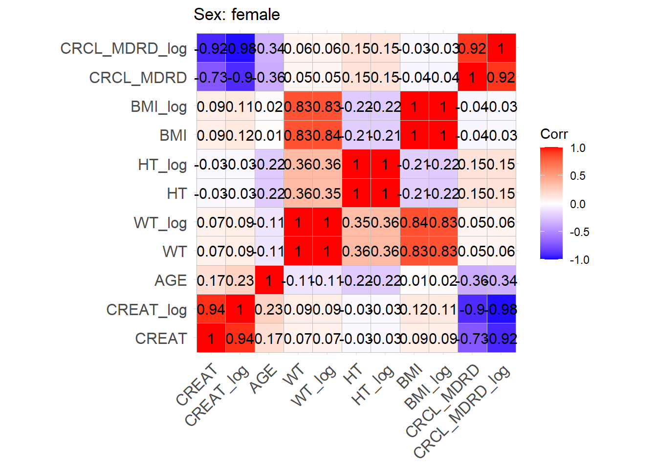
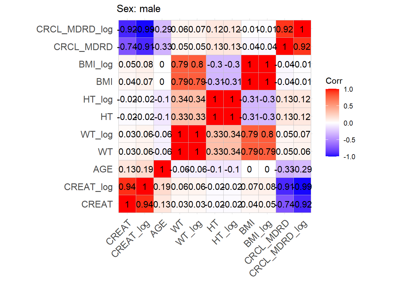
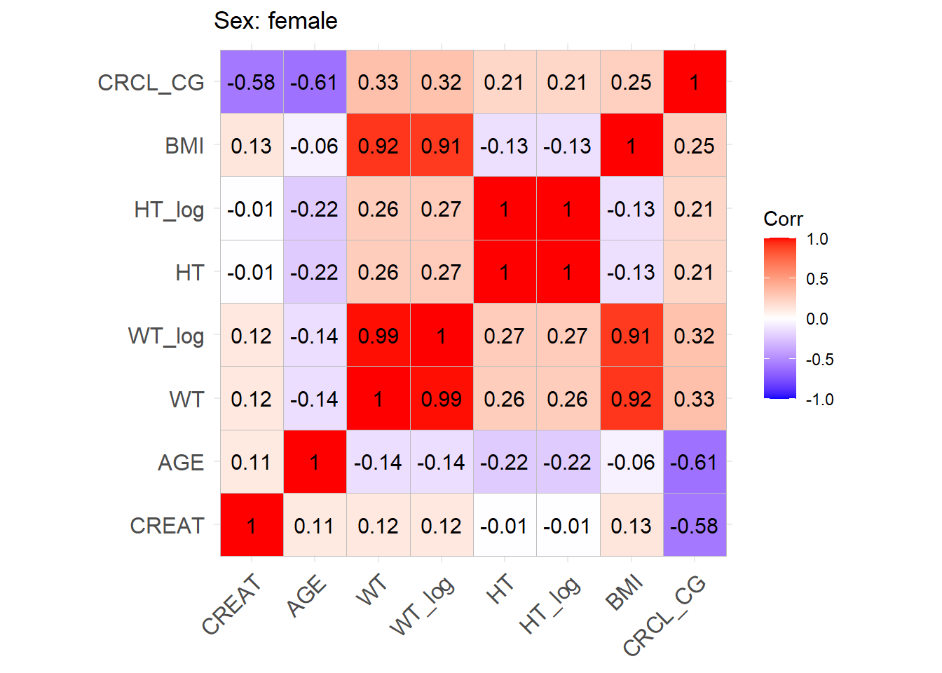
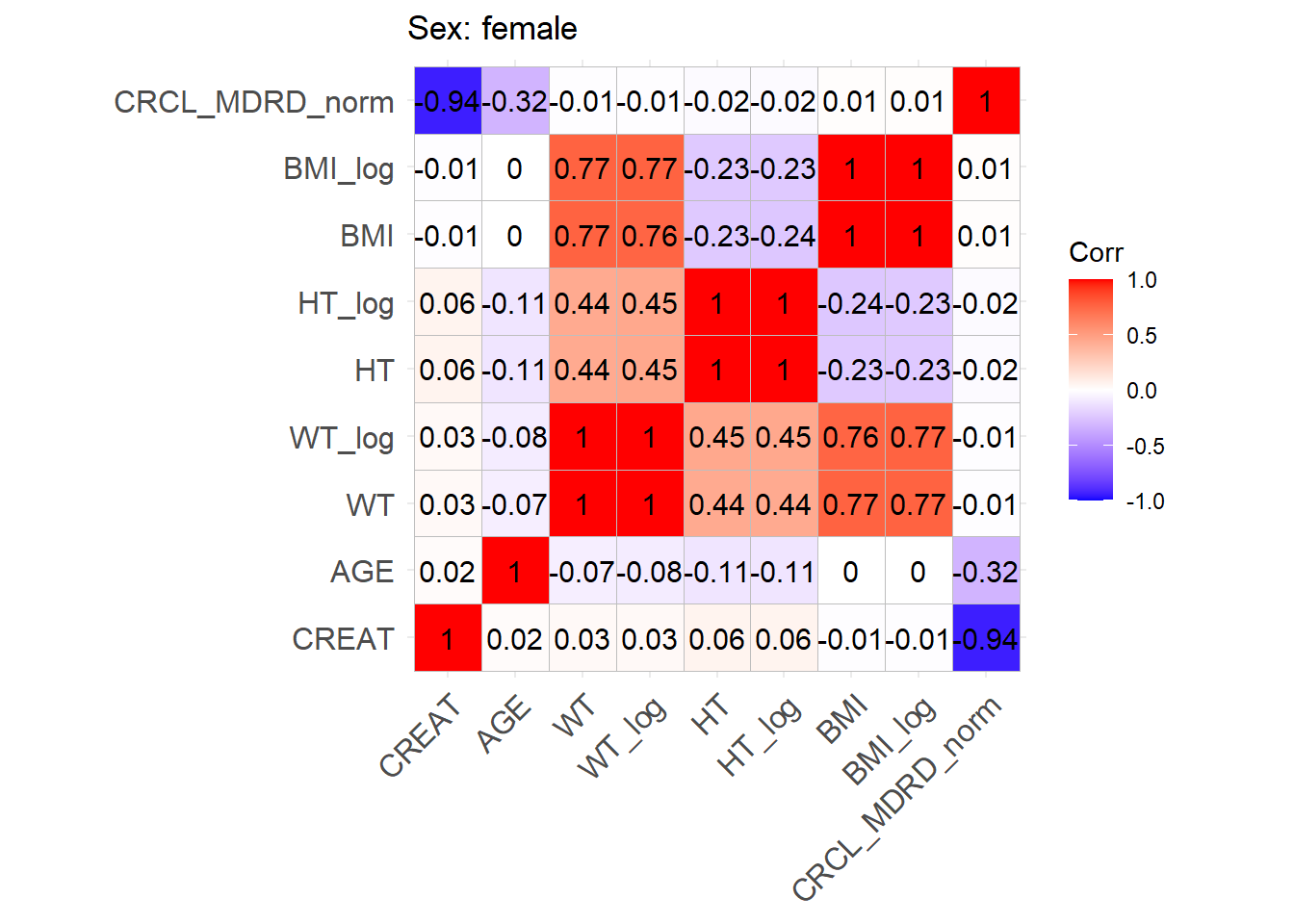
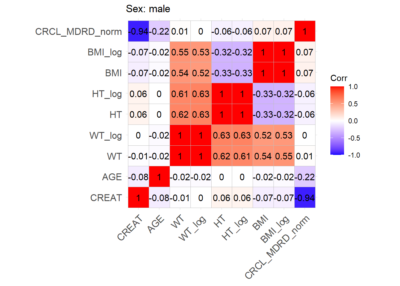
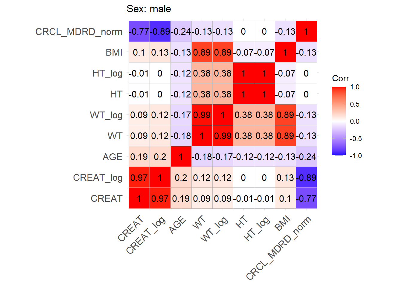
One issue with the covariate data reported in these papers is that correlations between covariates are not reported and simulating without correlations runs the risk of simulating improbable covariate values. We thus obtained a clinical dataset composed of more than 16000 ICU patients (Johnson et al. (2023)) from which we could derive correlations between covariates of interest. Age, serum creatinine, body weight, sex, height and BMI were obtained for these patients and the creatinine clearance was calculated (in mL/min for Cockroft and Gault and CKD-EPI and in mL/min/1.73 m2 for MDRD (to correspond to Mellon)). A correlation matrix was calculated for each of the respective model development cohorts separately for females and males.

This correlation matrix is used to simulate correlations between the simulated WT, CRCL, AGE, and HT/BMI if necessary to convert CRCL to serum creatinine. (CRCL_MDRD_norm means CRCL in mL/min/1.73 m² used for Mellon and CRCL_MDRD in mL/min.). Different correlation matrices are used based on sex. This way two different mutltivariate distributions are simulated based on the two matrices with a number of patients that respects the original article proportions.

We can find correlations for the log-transforms of certain variables. For the covariates where a log-normal distribution fits better the log mean and standard deviation of this distribution will be used to sample log values with a multivariate normal distribution. At the end, the log variables will be retransformed to normal ones.

5.2 Carlier et al. (2013)

5.2.1 Covariate distribution

All patients are ICU patients and we will assume that they are not burn and not obese patients. Creatinine clearance was obtained using the measured urinary equation. Thus for all patients ICU = 1, BURN = 0.

As discussed in the article, renal replacement therapy is an exclusion criterion, therefore the minimum value of creatinine clearance is set to 10 mL/min, any simulated value below 10 mL/min will be resampled. CRCL was calculated using the measured urinary equation.

For WT and CRCL here are the data from the paper :

cov_data_carlier <- cov_data |> 
  filter(Paper == "Carlier_2013")

cov_data_carlier |> 
  filter(Covariate %in% c("WT","CRCL","AGE","BMI")) |> 
  kable()

Paper	Covariate	Unit	Median	Q1	Q3	Min	Max
Carlier_2013	WT	kg	75	70	79	NA	NA
Carlier_2013	CRCL	mL/min	102	50	157	10	NA
Carlier_2013	BMI	kg/m^{2}	24	21	25	NA	NA
Carlier_2013	AGE	year	62	58	72	NA	NA

cor_matrix_Carlier_F <- readRDS(here("Simulations/cor_matrix_Carlier_F.rds"))
print(cor_matrix_Carlier_F)

                    CREAT   CREAT_log         AGE          WT      WT_log
CREAT          1.00000000  0.93719806  0.17043554  0.07114115  0.07024583
CREAT_log      0.93719806  1.00000000  0.22904749  0.09016458  0.09019928
AGE            0.17043554  0.22904749  1.00000000 -0.11058359 -0.10874794
WT             0.07114115  0.09016458 -0.11058359  1.00000000  0.99663272
WT_log         0.07024583  0.09019928 -0.10874794  0.99663272  1.00000000
HT            -0.02615290 -0.03452481 -0.22145176  0.36158540  0.35423946
HT_log        -0.02656759 -0.03481661 -0.22200991  0.36341580  0.35641748
BMI            0.09120381  0.11653457  0.01416104  0.83213862  0.83590568
BMI_log        0.08905860  0.11477057  0.01748252  0.82644900  0.83409794
CRCL_MDRD     -0.73311938 -0.90200963 -0.35625197  0.05193539  0.05083450
CRCL_MDRD_log -0.91894029 -0.98323371 -0.33894619  0.05521443  0.05501799
                       HT      HT_log         BMI     BMI_log   CRCL_MDRD
CREAT         -0.02615290 -0.02656759  0.09120381  0.08905860 -0.73311938
CREAT_log     -0.03452481 -0.03481661  0.11653457  0.11477057 -0.90200963
AGE           -0.22145176 -0.22200991  0.01416104  0.01748252 -0.35625197
WT             0.36158540  0.36341580  0.83213862  0.82644900  0.05193539
WT_log         0.35423946  0.35641748  0.83590568  0.83409794  0.05083450
HT             1.00000000  0.99908709 -0.21054270 -0.21983890  0.15405745
HT_log         0.99908709  1.00000000 -0.20907388 -0.21810288  0.15428482
BMI           -0.21054270 -0.20907388  1.00000000  0.99655760 -0.03784624
BMI_log       -0.21983890 -0.21810288  0.99655760  1.00000000 -0.03799028
CRCL_MDRD      0.15405745  0.15428482 -0.03784624 -0.03799028  1.00000000
CRCL_MDRD_log  0.14873339  0.14934183 -0.03146339 -0.03070224  0.92275219
              CRCL_MDRD_log
CREAT           -0.91894029
CREAT_log       -0.98323371
AGE             -0.33894619
WT               0.05521443
WT_log           0.05501799
HT               0.14873339
HT_log           0.14934183
BMI             -0.03146339
BMI_log         -0.03070224
CRCL_MDRD        0.92275219
CRCL_MDRD_log    1.00000000

ggcorrplot(cor_matrix_Carlier_F, lab = TRUE, title = "Sex: female")

cor_matrix_Carlier_M <- readRDS(here("Simulations/cor_matrix_Carlier_M.rds"))
print(cor_matrix_Carlier_M)

                    CREAT   CREAT_log          AGE          WT      WT_log
CREAT          1.00000000  0.93656904  0.129584751  0.03477888  0.03489511
CREAT_log      0.93656904  1.00000000  0.191015858  0.06256888  0.06255796
AGE            0.12958475  0.19101586  1.000000000 -0.05978080 -0.05792048
WT             0.03477888  0.06256888 -0.059780801  1.00000000  0.99691085
WT_log         0.03489511  0.06255796 -0.057920475  0.99691085  1.00000000
HT            -0.01562634 -0.02015099 -0.099371429  0.33471772  0.33277207
HT_log        -0.01514335 -0.01943840 -0.098654543  0.33778296  0.33606644
BMI            0.04448518  0.07478234  0.002442579  0.78722872  0.78753911
BMI_log        0.04503665  0.07581809  0.004260007  0.79489820  0.79912510
CRCL_MDRD     -0.73662552 -0.90639303 -0.327115476  0.04508957  0.04511819
CRCL_MDRD_log -0.92158994 -0.98613183 -0.287263519  0.06492902  0.06504475
                       HT      HT_log          BMI      BMI_log   CRCL_MDRD
CREAT         -0.01562634 -0.01514335  0.044485175  0.045036646 -0.73662552
CREAT_log     -0.02015099 -0.01943840  0.074782343  0.075818092 -0.90639303
AGE           -0.09937143 -0.09865454  0.002442579  0.004260007 -0.32711548
WT             0.33471772  0.33778296  0.787228725  0.794898201  0.04508957
WT_log         0.33277207  0.33606644  0.787539107  0.799125098  0.04511819
HT             1.00000000  0.99918214 -0.312182156 -0.300458114  0.12810278
HT_log         0.99918214  1.00000000 -0.309805459 -0.297640862  0.12729396
BMI           -0.31218216 -0.30980546  1.000000000  0.996020588 -0.03549251
BMI_log       -0.30045811 -0.29764086  0.996020588  1.000000000 -0.03551703
CRCL_MDRD      0.12810278  0.12729396 -0.035492514 -0.035517032  1.00000000
CRCL_MDRD_log  0.11829734  0.11791657 -0.010057809 -0.009333342  0.92462410
              CRCL_MDRD_log
CREAT          -0.921589942
CREAT_log      -0.986131825
AGE            -0.287263519
WT              0.064929019
WT_log          0.065044752
HT              0.118297341
HT_log          0.117916569
BMI            -0.010057809
BMI_log        -0.009333342
CRCL_MDRD       0.924624105
CRCL_MDRD_log   1.000000000

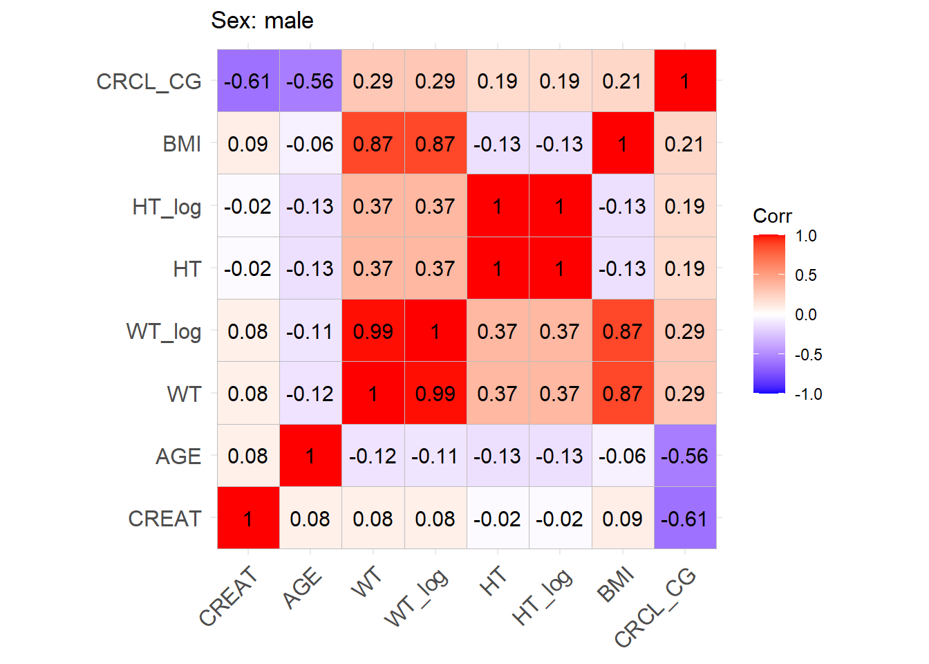
ggcorrplot(cor_matrix_Carlier_M, lab = TRUE, title = "Sex: male")

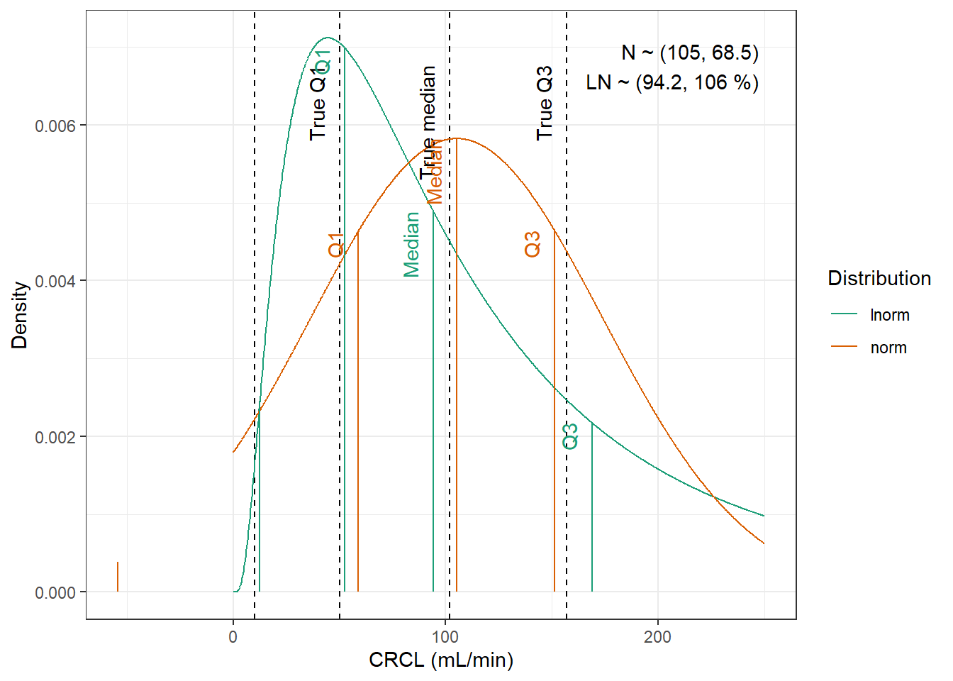
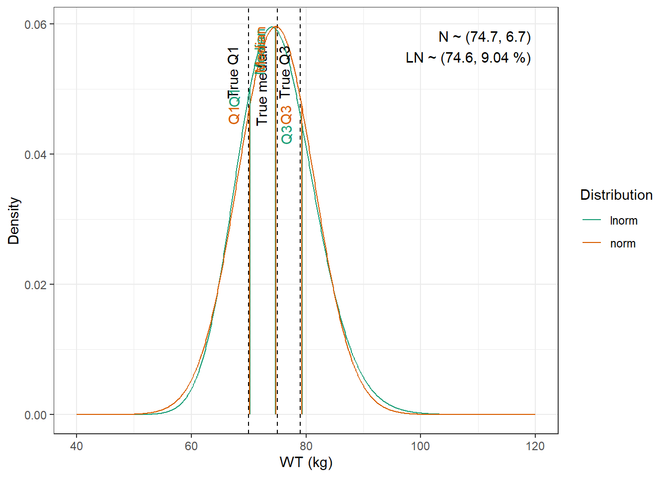
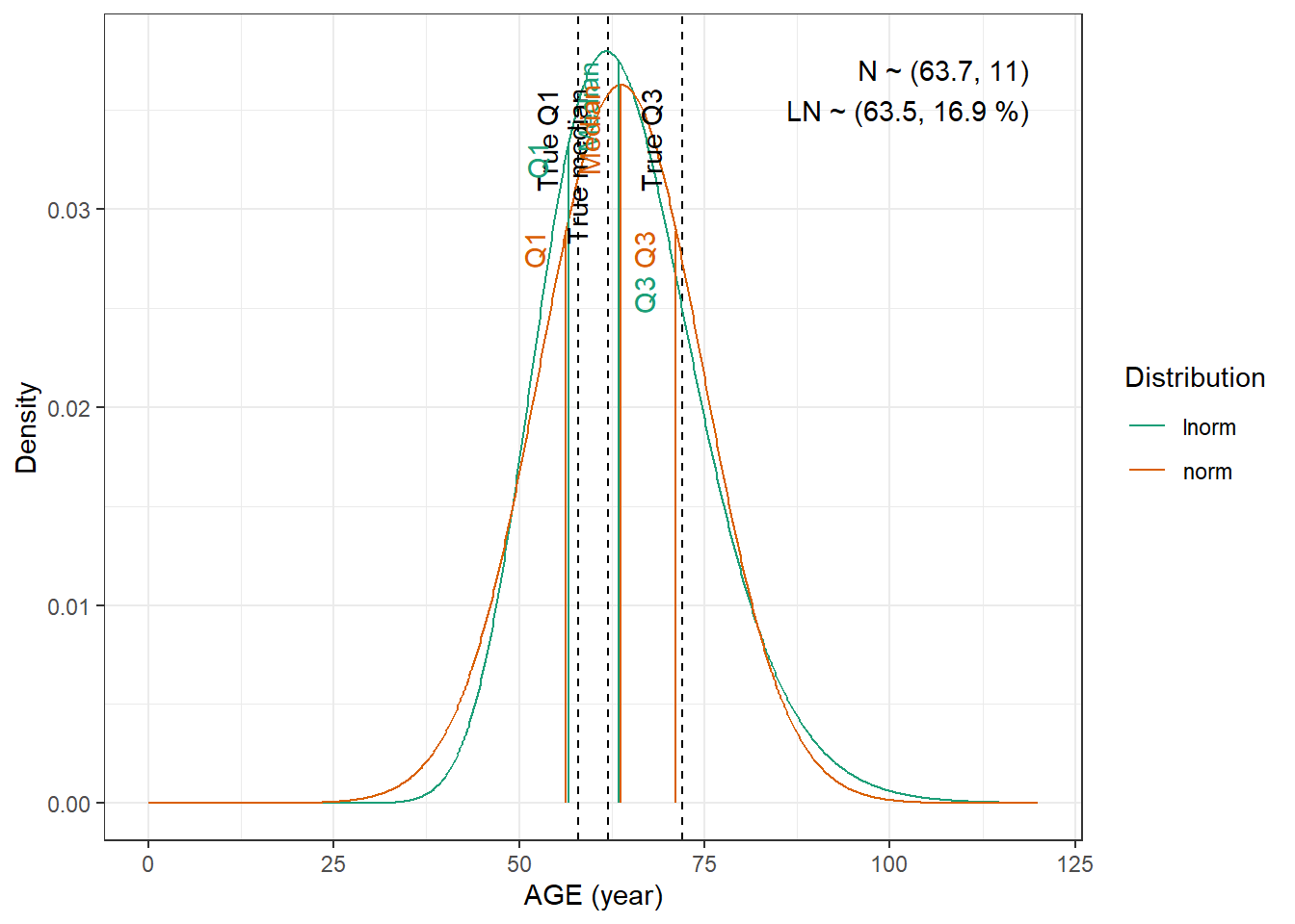
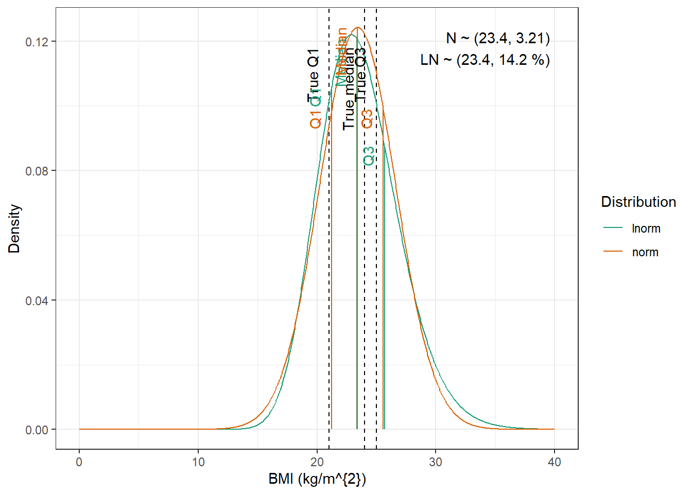
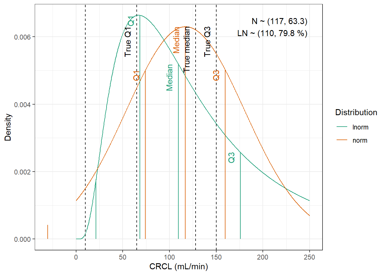
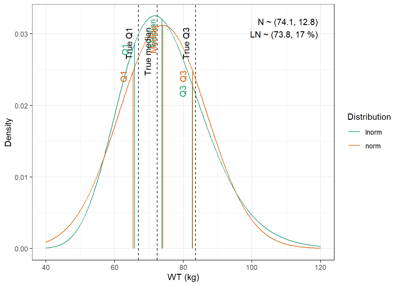
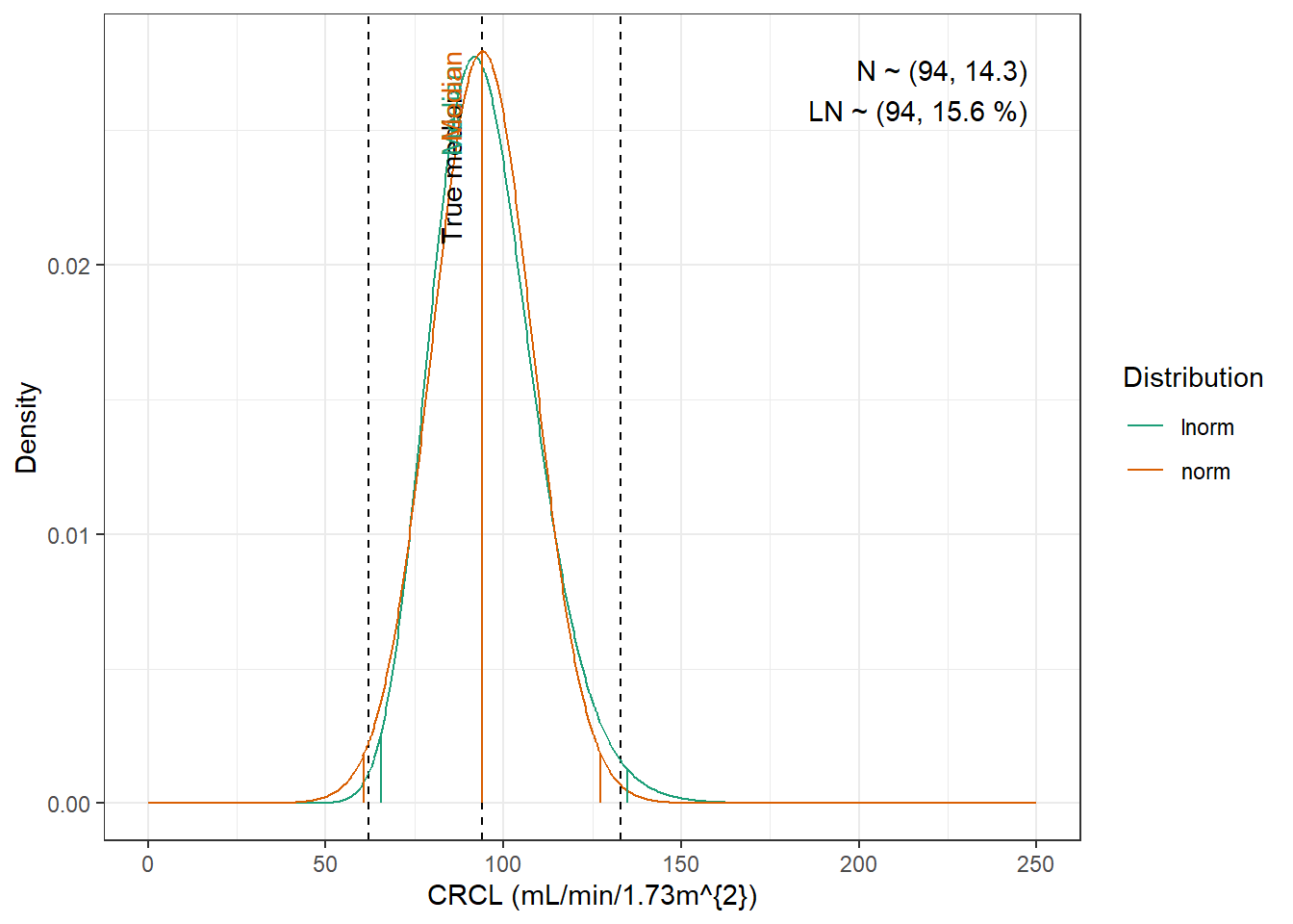
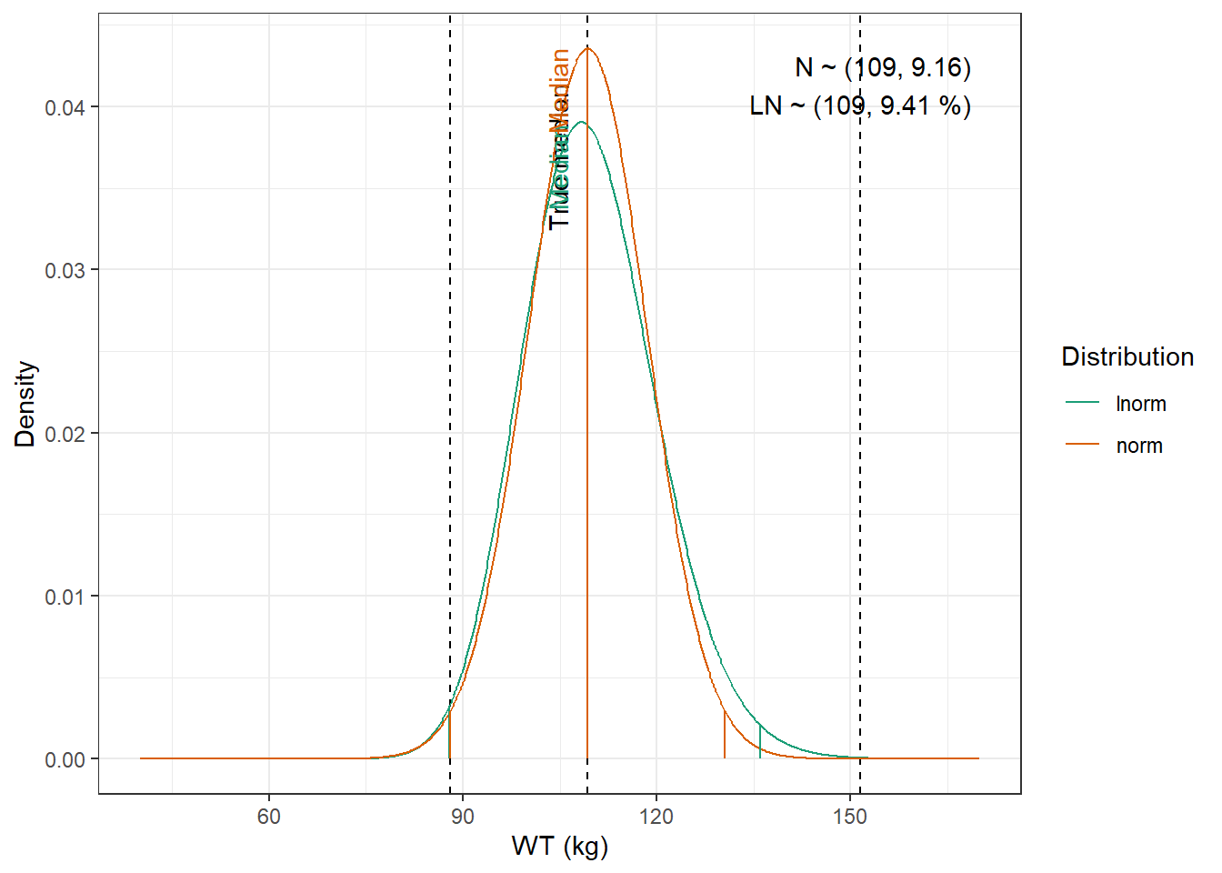
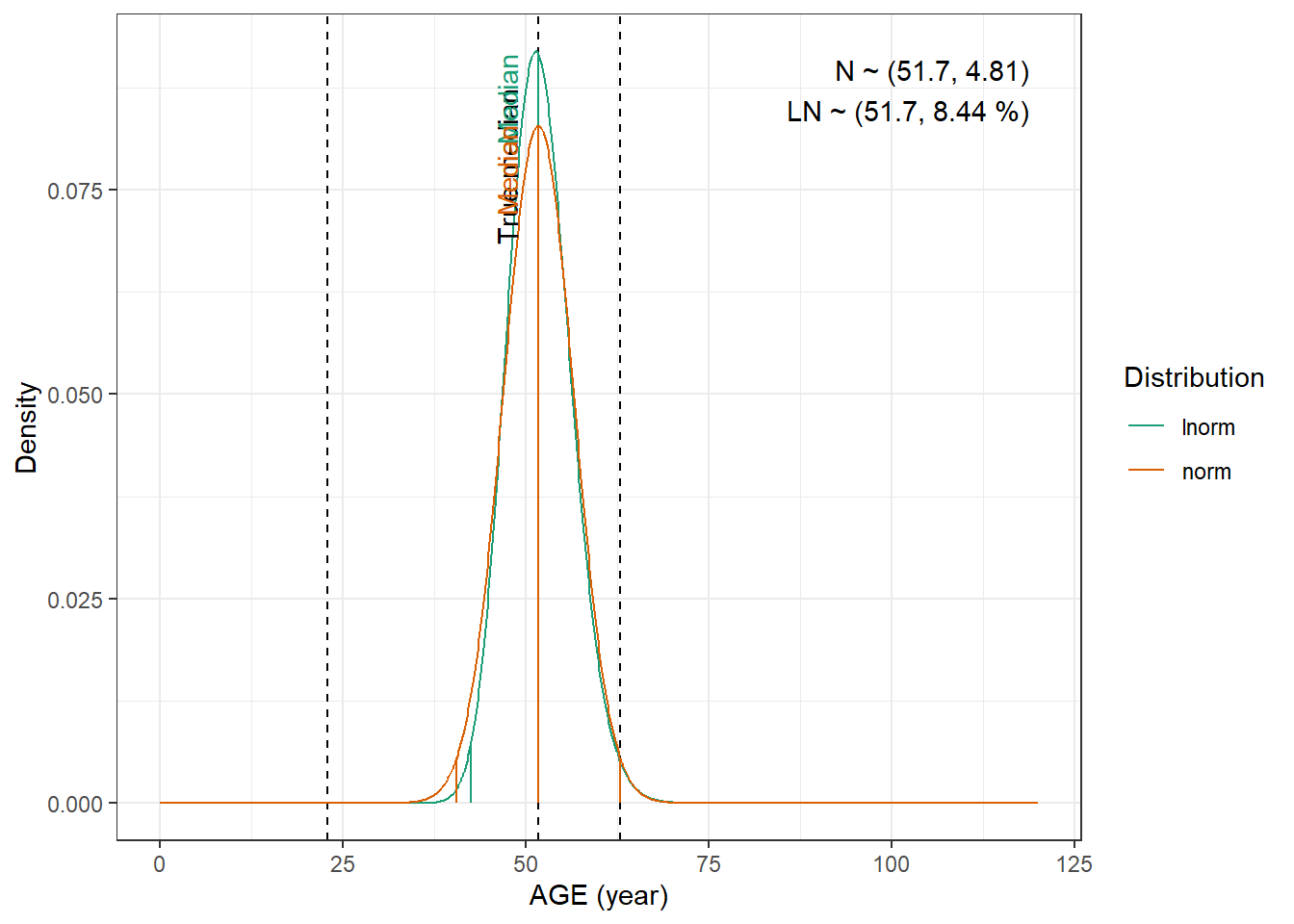
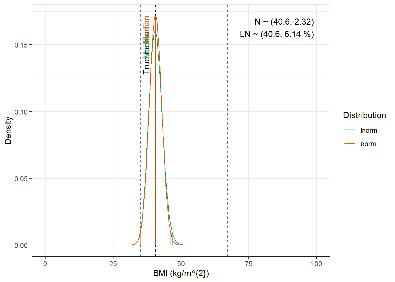
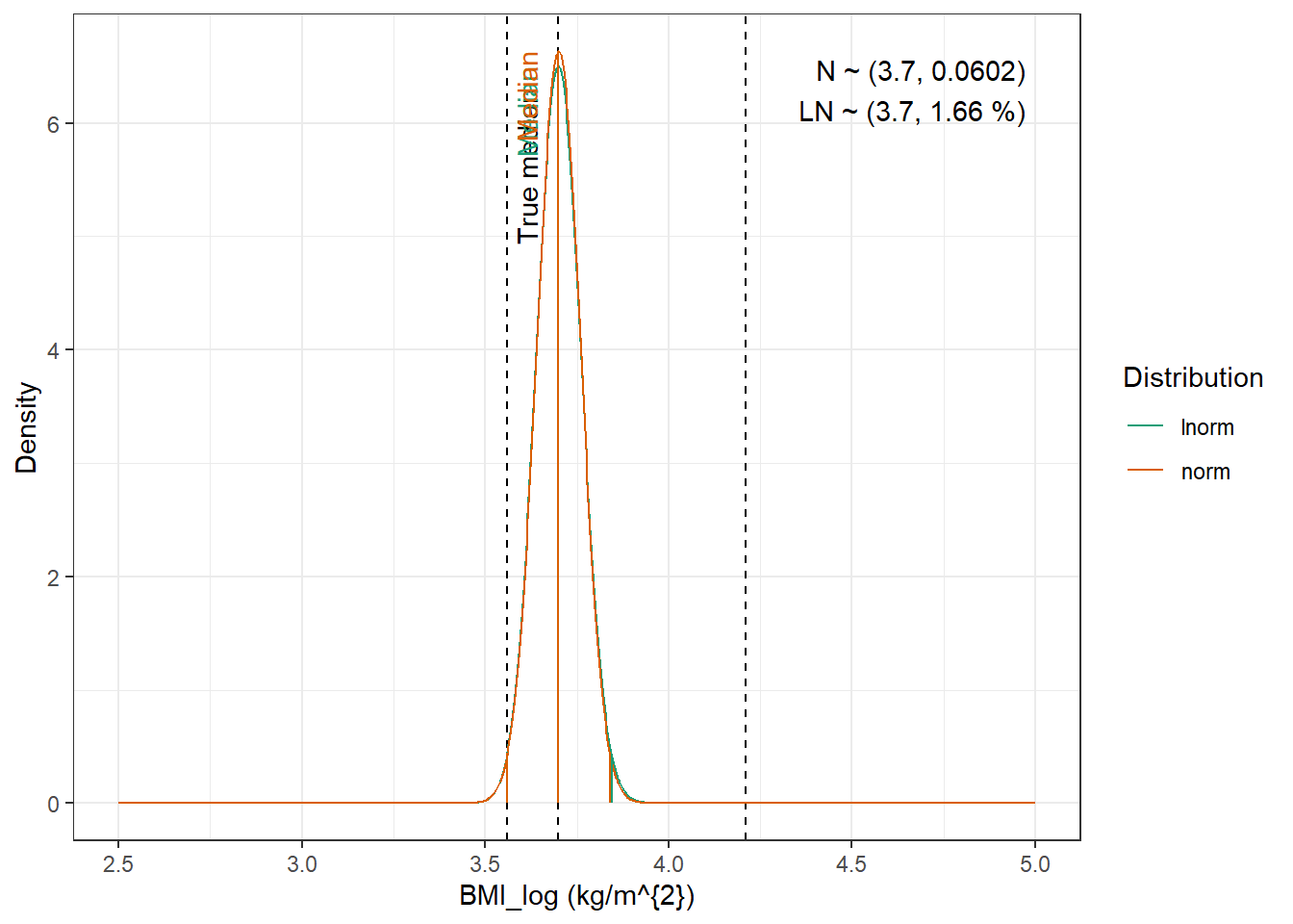
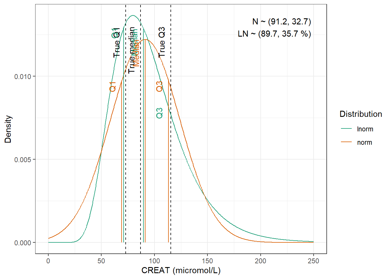
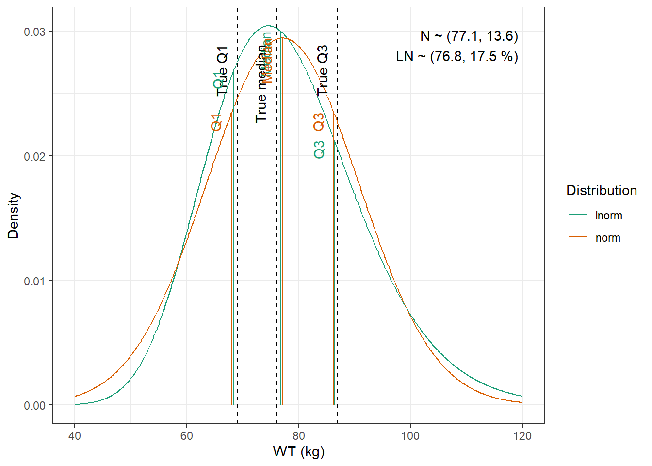
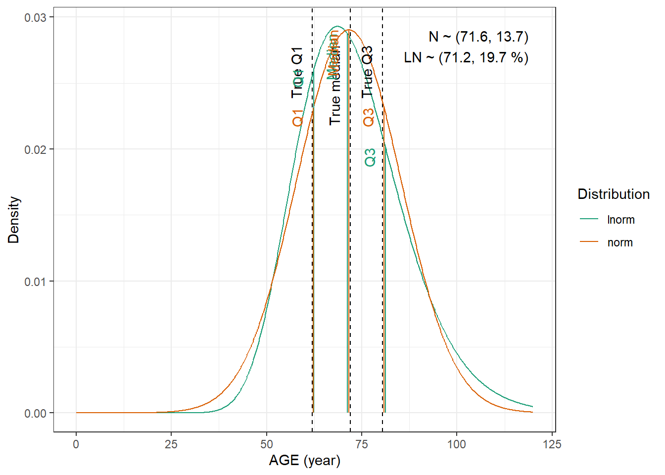
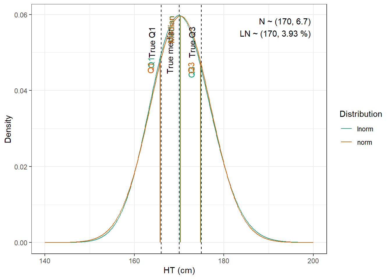
We are going to fit normal and log-normal distributions to the observed quantiles and select the best fitting one

compute_cv_from_sd_lnorm <- function(sdlog){
  #' Compute the geometric coefficient of variation from the standard deviation of a lognormal distribution
  #'
  #' @param sdlog numeric. standard deviation of the log transformed variable
  #' 
  #' @return numeric. geometric coefficient of variation
  sqrt(exp(sdlog^2)-1)
}

extract_cov_param <- function(cov_data, cov_name) {
  
  #' Get covariate quantiles from covariate characteristics table
  #'
  #' @param cov_data tibble containing the covariate information
  #' @param cov_name character. name of the covariate to select, comes from the Covariate column of cov_data.
  #' @return list with :
  #'  - p : numeric vector of probabilities
  #'  - q : numeric vector of quantiles
  #'  - cov_name : character string containing the covariate name
  #'  - cov_unit : character string containing the unit of the covariate
  
  
  cov_filtered_df <- cov_data |>
    filter(Covariate == cov_name) |>
    pivot_longer(
      cols = c(Median, Q1, Q3, Min, Max), # if the format of the csv columns ever changes, this will need to change
      names_to = "p",
      values_to = "q"
    ) |>
    mutate(p = case_match(p, "Median" ~ 0.5, "Q1" ~ 0.25, "Q3" ~ 0.75, "Min" ~ 0.01, "Max" ~ 0.99)) |>
    # if the format of the csv columns ever changes, the code above will need to change
    filter(!is.na(q)) |>
    group_by(Paper) |>
    arrange(p, .by_group = TRUE) |>
    ungroup()
  
  list(
    p = cov_filtered_df$p,
    q = cov_filtered_df$q,
    cov_name = unique(cov_filtered_df$Covariate),
    cov_unit = unique(cov_filtered_df$Unit)
  )
  
  
}

evaluate_distrib <- function(p, q, cov_name, cov_unit, min_plot, max_plot,tol = 0.001) {
  #' Fit normal and lognormal distribution to observed quantiles
  #' @param p numeric vector of probabilities
  #' @param q numeric vector of quantiles
  #' @param cov_name character string containing the covariate name
  #' @param cov_unit character string containing the unit of the covariate
  #' @param min_plot minimal value of the covariate for which the distribution should be plotted
  #' @param max_plot maximal value of the covariate for which the distribution should be plotted
  #' @param tol numeric. tolerance value for the fitting algorithm, default is 0.001
  #' @return list with :
  #'  - plot : ggplot2 showing the fitted distributions and the observed covariate
  #'  - lnorm_par : named numeric vector with the lognormal distribution parameters
  #'  - norm_par : named numeric vector with the normal distribution parameters
  
  
  lnorm_par <- get.lnorm.par(p = p, q = q, plot = FALSE, show.output = FALSE,tol = tol)
  norm_par <- get.norm.par(p = p, q = q, plot = FALSE, show.output = FALSE,tol=tol)
  
  #create a dataset with the true percentiles to be able to show them on the plot
  true_percentiles <- tibble(p, q) |> 
    mutate(label = case_match(p, 
                              0 ~ "True min",
                              0.25 ~ "True Q1",
                              0.5 ~ "True median",
                              0.75 ~ "True Q3",
                              1 ~ "True max")) 
  
  #create a dataset with the percentiles of the fitted distributiosn to be able to show them on the plot
  distrib_percentiles <-  tibble(
    probability = p,
    lnorm = qlnorm(probability, meanlog = lnorm_par["meanlog"], sdlog =
                     lnorm_par["sdlog"]),
    norm = qnorm(probability, mean = norm_par["mean"], sd = norm_par["sd"])
  ) |>
    pivot_longer(cols = c(lnorm, norm), names_to = "distrib") |>
    mutate(density = case_match(
      distrib,
      "norm" ~ dnorm(value, mean = norm_par["mean"], sd =
                       norm_par["sd"]),
      "lnorm" ~ dlnorm(value, meanlog = lnorm_par["meanlog"], sdlog =
                         lnorm_par["sdlog"])
    )) |> 
    mutate(label = case_match(probability, 
                              0 ~ "Min",
                              0.25 ~ "Q1",
                              0.5 ~ "Median",
                              0.75 ~ "Q3",
                              1 ~ "Max")) 
  
  
  #simulate 1000 datapoints from the fitted distributions to show on the plot
  param_data <- tibble(
    variable = seq(min_plot, max_plot, length.out = 1000),
    lnorm = dlnorm(variable, meanlog = lnorm_par["meanlog"], sdlog = lnorm_par["sdlog"]),
    norm = dnorm(variable, mean = norm_par["mean"], sd = norm_par["sd"])
  ) |>
    pivot_longer(cols = c(lnorm, norm), names_to = "distrib")
  
  
  plot <- ggplot(param_data, aes(x = variable, y = value, color = distrib)) +
    geom_vline(data = true_percentiles, mapping = aes(xintercept = q),lty = "dashed") +
    geom_line() +
    geom_segment(data = distrib_percentiles, aes(x = value, y = 0, yend =
                                                   density)) +
    theme_bw() +
    scale_color_brewer("Distribution", palette = "Dark2") +
    ylab("Density") +
    xlab(paste0(cov_name, " (", cov_unit, ")")) +
    annotate(
      geom = "text",
      label = paste0(
        "N ~ (",
        signif(norm_par["mean"], 3),
        ", ",
        signif(norm_par["sd"], 3),
        ")\n",
        "LN ~ (",
        signif(exp(lnorm_par["meanlog"]), 3),
        ", ",
        signif(compute_cv_from_sd_lnorm(lnorm_par["sdlog"]), 3) * 100,
        " %)"
      ),
      x = min(param_data$variable) + 0.99 * diff(range(param_data$variable)),
      y = min(param_data$value) + 0.99 * diff(range(param_data$value)),
      hjust = 1,
      vjust = 1
    )+
    geom_text(
      data = true_percentiles,
      mapping = aes(x = q,label = label,color=NULL),
      show.legend = FALSE,
      y = min(param_data$value) + 0.95 * diff(range(param_data$value)),
      hjust = 1,
      vjust = -1,
      angle = 90
    )+
    geom_text(
      data = distrib_percentiles,
      mapping = aes(x = value, y=density,label = label),
      show.legend = FALSE,
      hjust = 1,
      vjust = -1,
      angle = 90
    )
  
  list(plot = plot,
       lnorm_par = lnorm_par,
       norm_par = norm_par)
  
}

fit_cov_wrapper <- function(cov_data, cov_name, min_plot, max_plot, tol = 0.001) {
  
  #' Wrapper to get covariate quantiles from covariate characteristics table and fit normal and lognormal distribution
  #' to observed quantiles 
  #'
  #' @param cov_data tibble containing the covariate information
  #' @param cov_name character. name of the covariate to select, comes from the Covariate column of cov_data.
  #' @param min_plot minimal value of the covariate for which the distribution should be plotted
  #' @param max_plot maximal value of the covariate for which the distribution should be plotted
  #' @param tol numeric. tolerance value for the fitting algorithm, default is 0.001
  #' @return list with :
  #'  - plot : ggplot2 showing the fitted distributions and the observed covariate
  #'  - lnorm_par : named numeric vector with the lognormal distribution parameters
  #'  - norm_par : named numeric vector with the normal distribution parameters
  
  
  cov_df <- extract_cov_param(cov_data, cov_name)
  
  evaluate_distrib(
    p = cov_df$p,
    q = cov_df$q,
    min_plot = min_plot,
    max_plot = max_plot,
    cov_name = cov_df$cov_name,
    cov_unit = cov_df$cov_unit,
    tol = tol
  )
  
}

carlier_crcl <- fit_cov_wrapper(
  cov_data = cov_data_carlier,
  cov_name = "CRCL",
  min_plot = 0,
  max_plot = 250
)

carlier_crcl$plot

Normal distribution seems better than log-normal.

carlier_wt <- fit_cov_wrapper(
  cov_data = cov_data_carlier,
  cov_name = "WT",
  min_plot = 40,
  max_plot = 120
)

carlier_wt$plot

No discernable difference in fit. We have to use the log-normal distribution to be able to calculate height.

carlier_age <- fit_cov_wrapper(
  cov_data = cov_data_carlier,
  cov_name = "AGE",
  min_plot = 0,
  max_plot = 120
)

carlier_age$plot

No discernible difference in fit. We will use the normal distribution as generally, age is normally distributed.

carlier_bmi <- fit_cov_wrapper(
  cov_data = cov_data_carlier,
  cov_name = "BMI",
  min_plot = 0,
  max_plot = 40,
  tol=0.002
)

carlier_bmi$plot

Tolerance was increased to 0.002. No discernible difference in fit. We have to use the log-normal distribution to be able to obtain height.

5.2.2 Simulation of covariates

Covariates will be sampled from the following distributions :

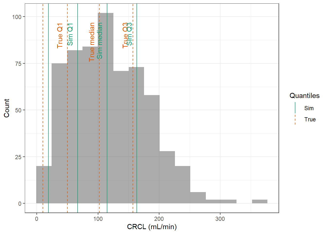
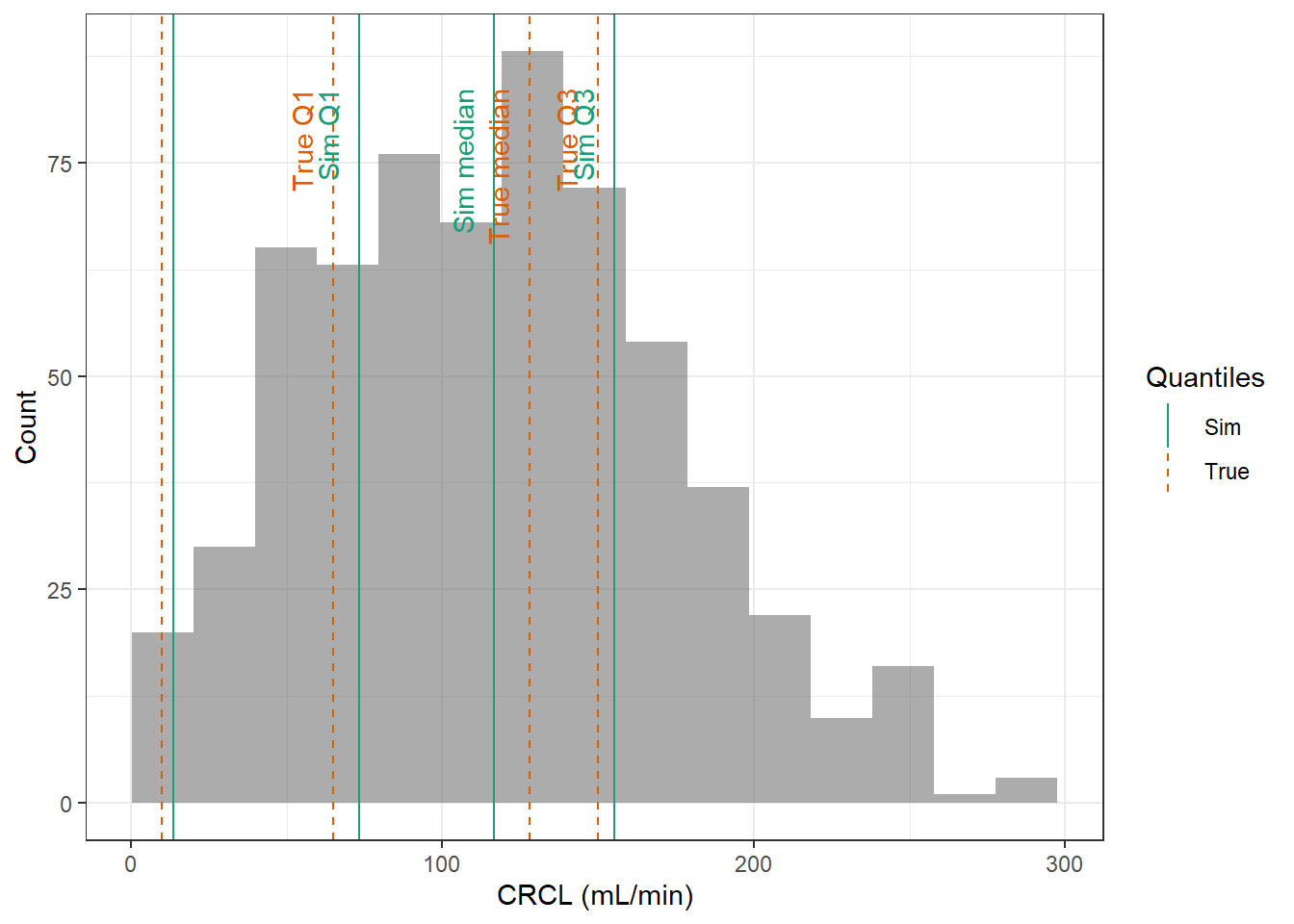
• CRCL : Normal distribution with a minimum of 10 mL/min, with mean 105 mL/min and standard deviation 68.5 mL/min
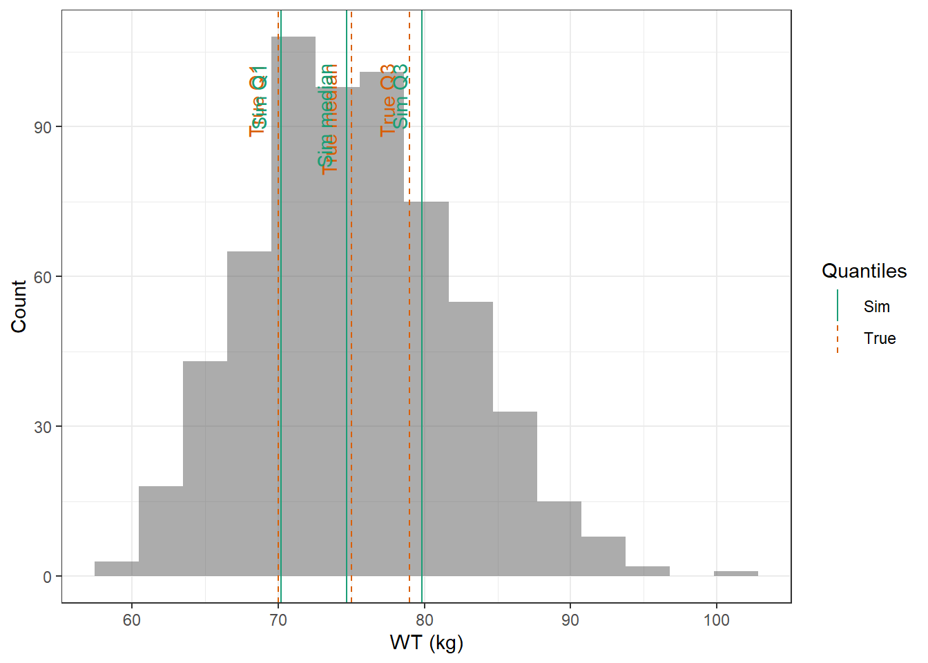
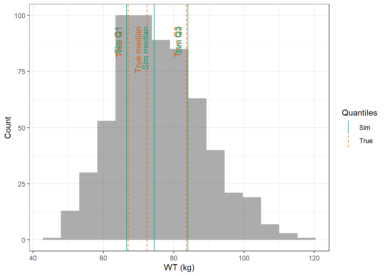
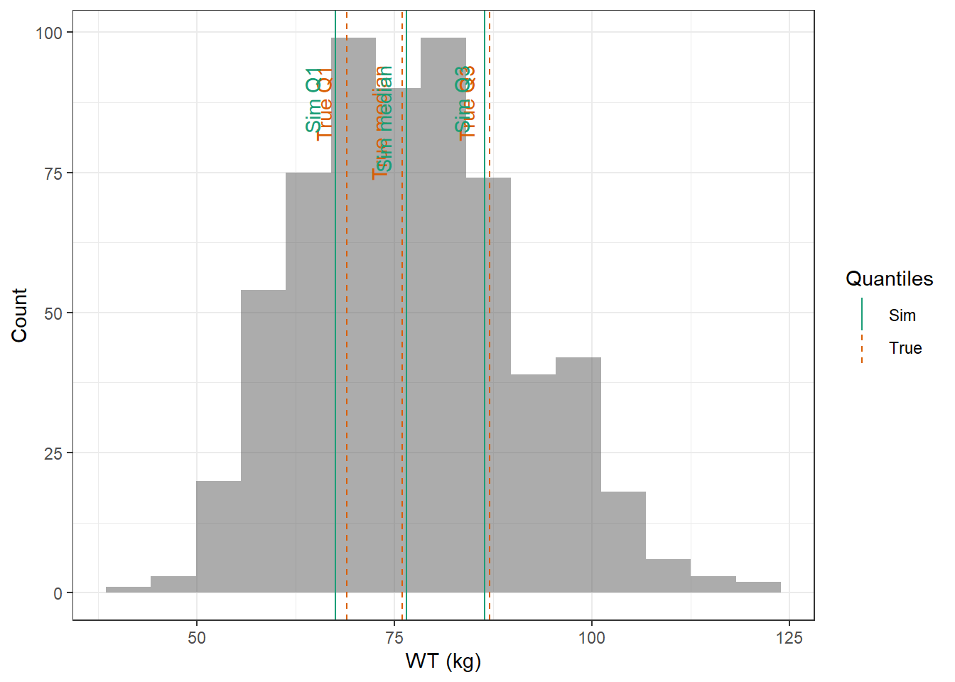
• WT : Lognormal distribution with mean 74.6 kg, and coefficient of variation 9.04 %
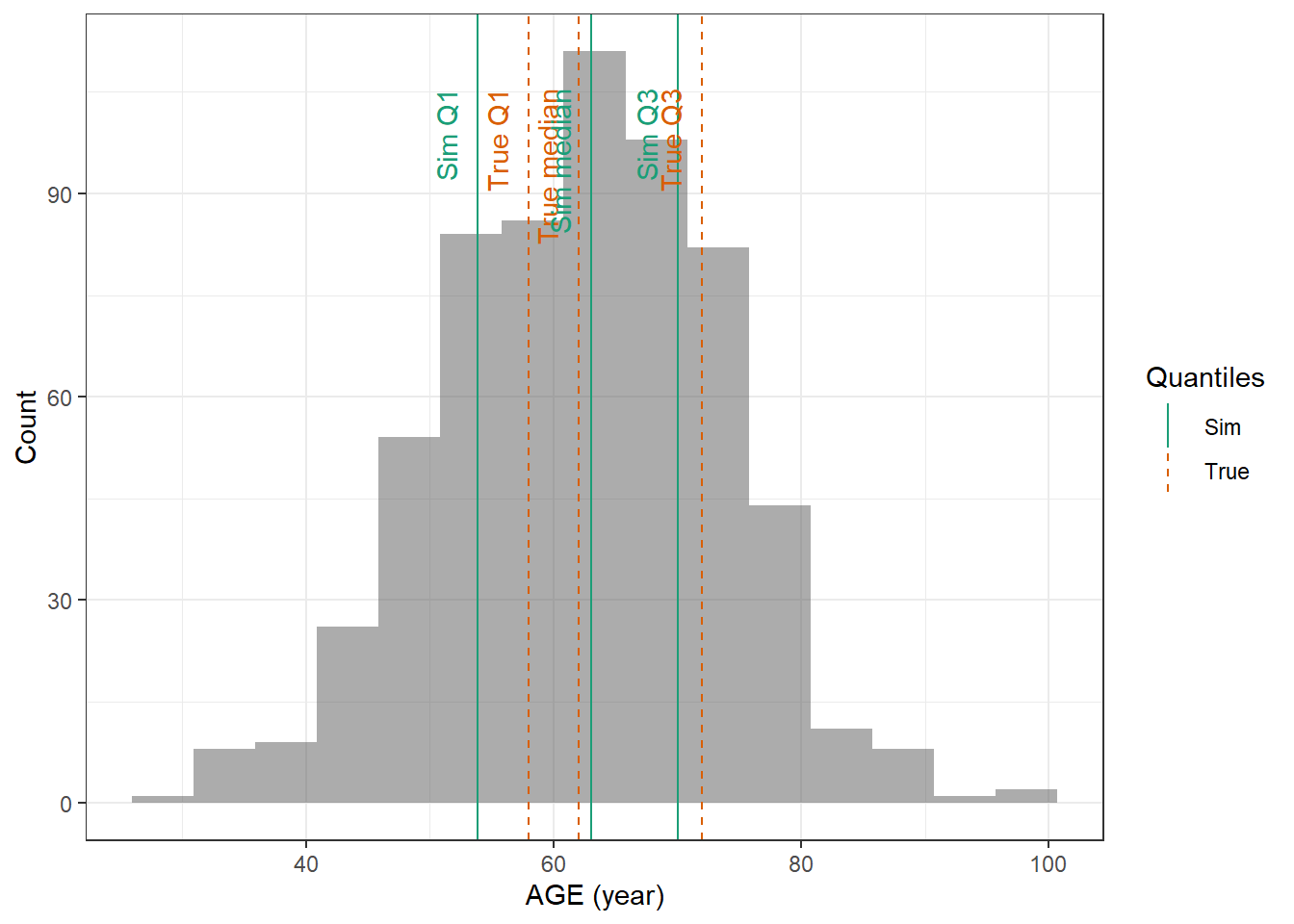
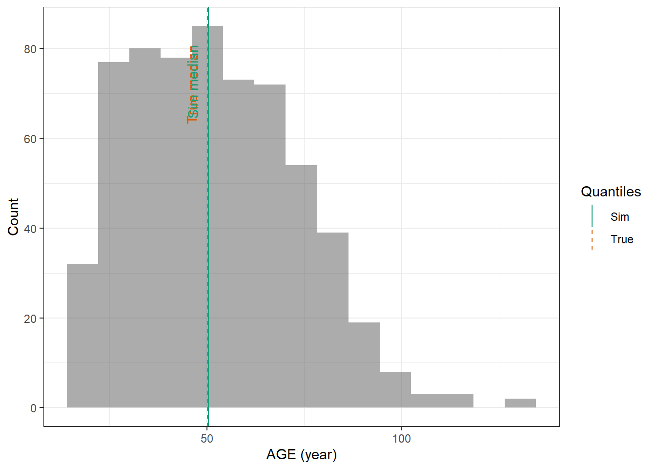
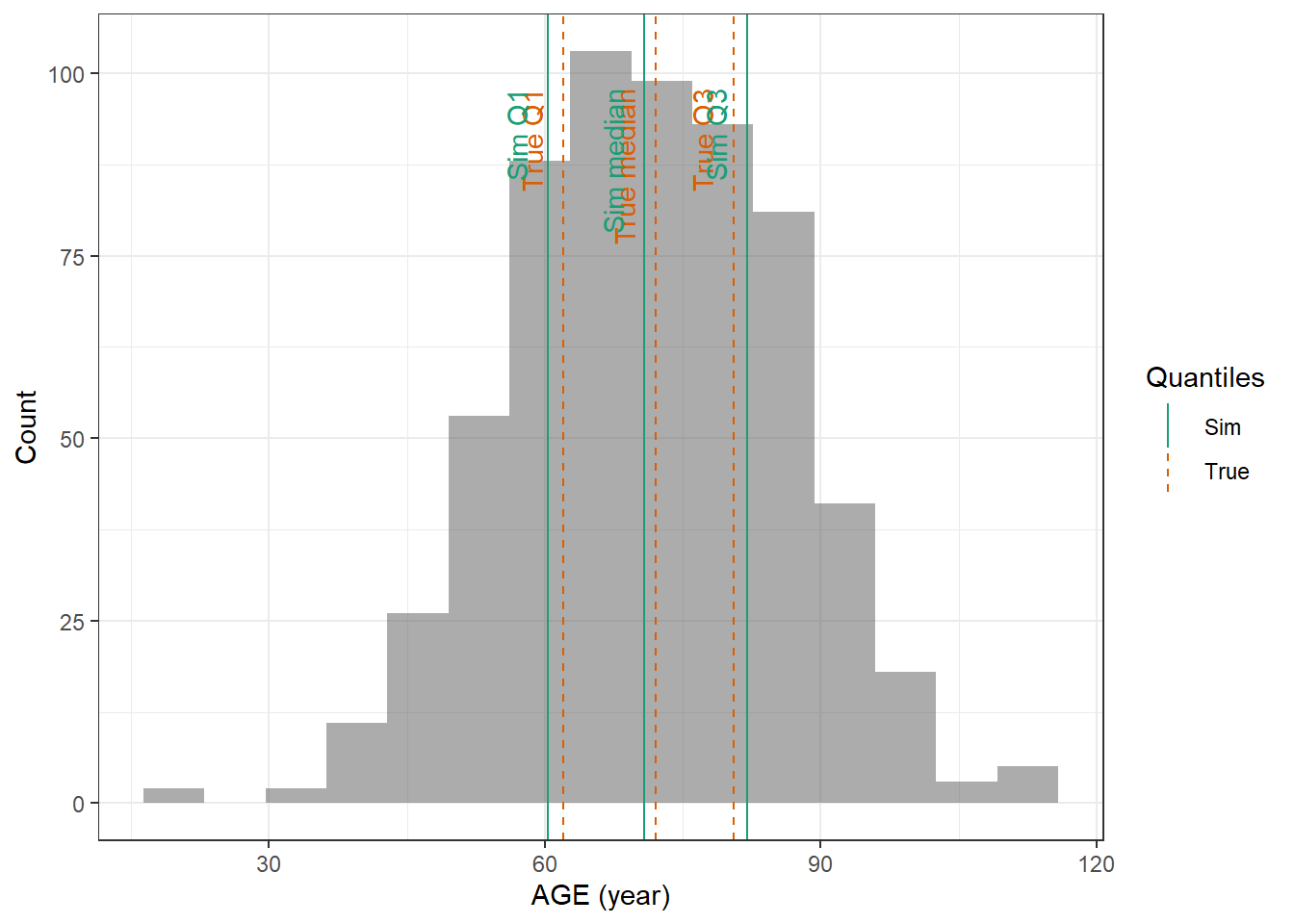
• AGE : Normal distribution with mean 63.7 mL/min and standard deviation 11 years and with a minimum of 18 years
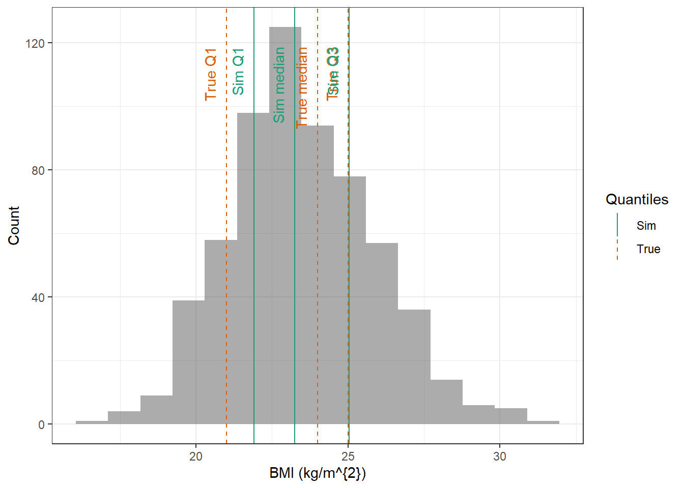
• BMI : Log-normal distribution with mean 3.15 mL/min and standard deviation 0.141 kg/m^{2}

sim_norm_without_negatives <- function(n,mean,sd){
      
  #' Simulate values from normal distribution but resample negative values
  #'
  #' @param n numeric. number of samples to simulate
  #' @param mean numeric. mean of the normal distribution
  #' @param sd numeric. standard deviation of the normal distribtuion
  #' @return numeric vector of n values
  sim_values <- rnorm(n,mean,sd)
  neg_values <- sim_values[sim_values<=0]
  pos_values <- sim_values[sim_values>0]

  while(length(neg_values)>0){
    new_values <- rnorm(length(neg_values),mean,sd)
    sim_values <- c(pos_values,new_values)
    neg_values <- sim_values[sim_values<=0]
    pos_values <- sim_values[sim_values>0]
    }
  sim_values
}

# Only for normal distribution when the minimum is 10 ml/min, resample below 10
sim_norm_without_dialysis <- function(n,mean,sd){
      
  #' Simulate values from normal distribution but resample negative values
  #'
  #' @param n numeric. number of samples to simulate
  #' @param mean numeric. mean of the normal distribution
  #' @param sd numeric. standard deviation of the normal distribtuion
  #' @return numeric vector of n values
  sim_values <- rnorm(n,mean,sd)
  neg_values <- sim_values[sim_values<=10]
  pos_values <- sim_values[sim_values>10]

  while(length(neg_values)>0){
    new_values <- rnorm(length(neg_values),mean,sd)
    sim_values <- c(pos_values,new_values)
    neg_values <- sim_values[sim_values<=10]
    pos_values <- sim_values[sim_values>10]
    }
  sim_values
}
# Resimulate subjects younger than 18 years for normally distributed age
sim_norm_without_minors <- function(n,mean,sd){
      
  #' Simulate values from normal distribution but resample negative values
  #'
  #' @param n numeric. number of samples to simulate
  #' @param mean numeric. mean of the normal distribution
  #' @param sd numeric. standard deviation of the normal distribtuion
  #' @return numeric vector of n values
  sim_values <- rnorm(n,mean,sd)
  neg_values <- sim_values[sim_values<18]
  pos_values <- sim_values[sim_values>=18]

  while(length(neg_values)>0){
    new_values <- rnorm(length(neg_values),mean,sd)
    sim_values <- c(pos_values,new_values)
    neg_values <- sim_values[sim_values<18]
    pos_values <- sim_values[sim_values>=18]
    }
  sim_values
}

The relevant part of the correlation matrix is converted to a covariance matrix by multiplying the already calculated standard deviations of the variables with the diagonal of the correlation matrix. More information can be found at SAS and at stats. A multivariate normal distribution is fitted with resimulation of CRCL below 10 ml/min, AGE below 18 years, and other variables below 0.

The proportion of males is 0.85 in the original article, so the number of males is 531 and the number of females is 94 to add up to 625.

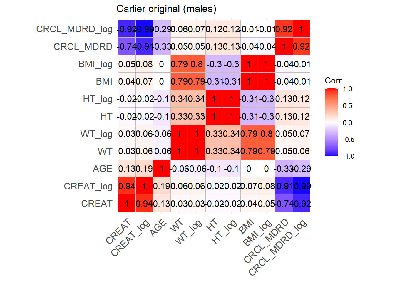
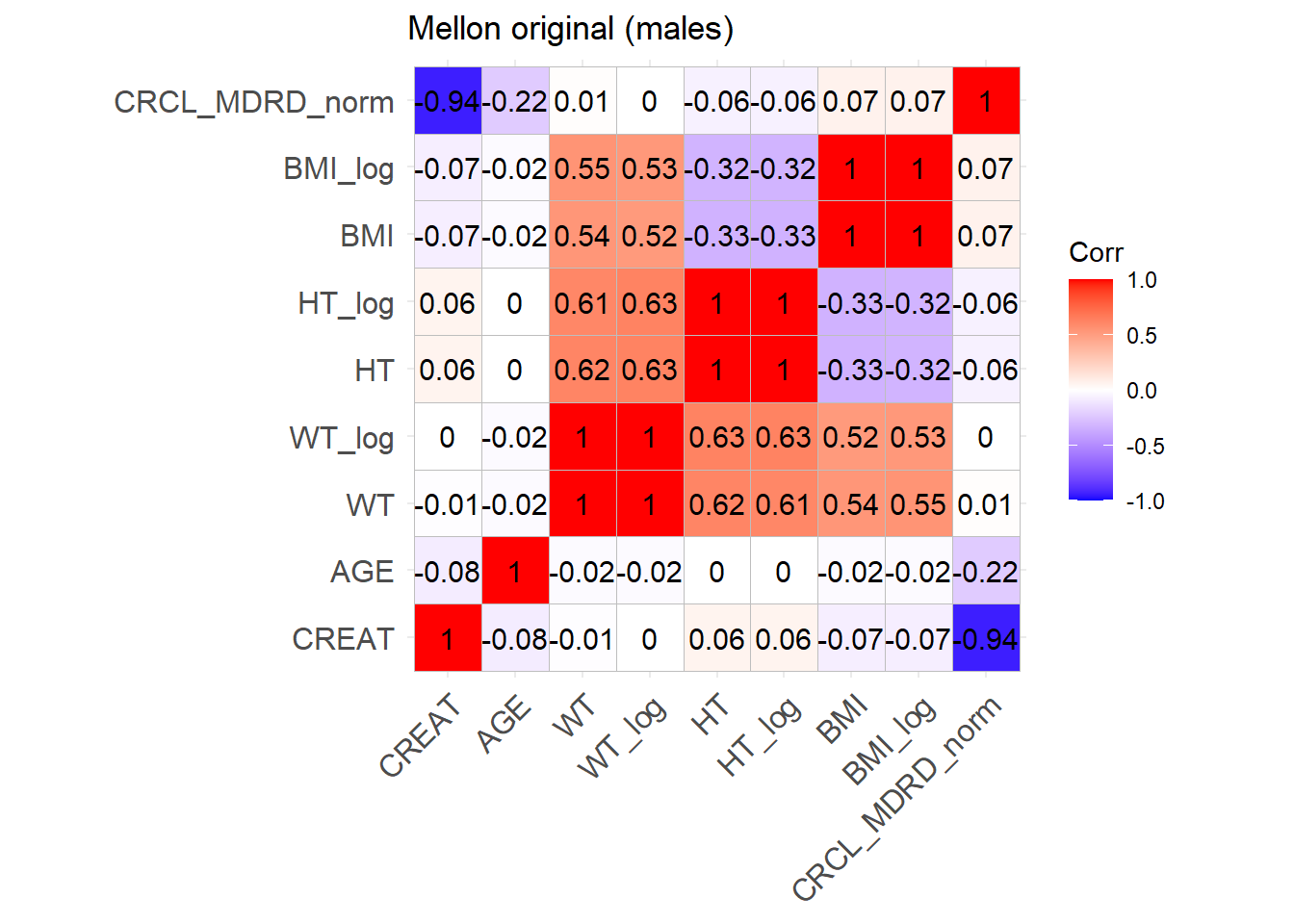
mean_WT_log <- as.numeric(carlier_wt$lnorm_par["meanlog"])
sd_WT_log <- as.numeric(carlier_wt$lnorm_par["sdlog"])
mean_BMI_log <- as.numeric(carlier_bmi$lnorm_par["meanlog"])
sd_BMI_log <- as.numeric(carlier_bmi$lnorm_par["sdlog"])
r_M <- 0.34 # Pearson correlation between HT_log and WT_log for males
r_F <- 0.36 # Pearson correlation for females

# sd is different based on sex
mean_HT_log = (mean_WT_log - mean_BMI_log) / 2
sd_HT_M_log = (-r_M * sd_WT_log + sqrt(r_M^2 * sd_WT_log^2 - sd_WT_log^2 + sd_BMI_log^2))/2 # quadratic equation with positive result
sd_HT_F_log = (-r_F * sd_WT_log + sqrt(r_F^2 * sd_WT_log^2 - sd_WT_log^2 + sd_BMI_log^2))/2 # quadratic equation with positive

correlated_simulation <- function(n, means, cov_matrix) {
  set.seed(1991)
  collected <- matrix(NA, 0, length(means))
  colnames(collected) <- names(means)

  while (nrow(collected) < n) {
    batch <- MASS::mvrnorm(n = n, mu = means, Sigma = cov_matrix)
    colnames(batch) <- names(means)

    valid <- batch[, "AGE"] >= 18 &
             batch[, "CRCL_MDRD"] >= 10

    batch_valid <- batch[valid, , drop = FALSE]
    collected <- rbind(collected, batch_valid)
  }

  collected[1:n, , drop = FALSE]
}

means <- c(
  CRCL_MDRD = carlier_crcl$norm_par["mean"],
  WT_log      = carlier_wt$lnorm_par["meanlog"],
  AGE     = carlier_age$norm_par["mean"],
  HT_log     = mean_HT_log
)

sds_M <- c(
  CRCL_MDRD = carlier_crcl$norm_par["sd"],
  WT_log      = carlier_wt$lnorm_par["sdlog"], 
  AGE     = carlier_age$norm_par["sd"],
  HT_log     = sd_HT_M_log
)

sds_F <- c(
  CRCL_MDRD = carlier_crcl$norm_par["sd"],
  WT_log      = carlier_wt$lnorm_par["sdlog"], 
  AGE     = carlier_age$norm_par["sd"],
  HT_log     = sd_HT_F_log
)

covariates <- c("CRCL_MDRD", "WT_log", "AGE", "HT_log")

names(means) <- covariates

# Correlation and Covariance Matrix
cor_carlier_M <- cor_matrix_Carlier_M[covariates, covariates]
cov_matrix_M <- diag(sds_M) %*% cor_carlier_M %*% diag(sds_M)
eigen(cov_matrix_M)$values

[1] 4.705706e+03 1.077951e+02 8.326780e-03 1.446538e-03

cor_carlier_F <- cor_matrix_Carlier_F[covariates, covariates]
cov_matrix_F <- diag(sds_F) %*% cor_carlier_F %*% diag(sds_F)
eigen(cov_matrix_F)$values

[1] 4.708164e+03 1.053367e+02 8.259148e-03 1.338558e-03

# Simulate
sim_data_M <- correlated_simulation(n = 531, means = means, cov_matrix = cov_matrix_M)
sim_data_M <- as_tibble(sim_data_M) %>%
  mutate(SEX = 0)

sim_data_F <- correlated_simulation(n = 94, means = means, cov_matrix = cov_matrix_F)
sim_data_F <- as_tibble(sim_data_F) %>%
  mutate(SEX = 1)

sim_data <- rbind(sim_data_M, sim_data_F)

# Put the covariates together
sim_cov_carlier <- tibble(
  Paper = "Carlier_2013",
  ID_within_paper = 1:n_patient,
  ICU = 1,
  BURN = 0,
  OBESE = 0,
  CRCL = sim_data$CRCL_MDRD,
  WT_log   = sim_data$WT_log,
  AGE  = sim_data$AGE,
  HT_log  = sim_data$HT_log,
  SEX = sim_data$SEX
)

# Add OBESE variable and reconvert logWT to WT
sim_cov_carlier <- sim_cov_carlier %>%
  mutate(WT = exp(WT_log),
         HT = (exp(HT_log))*100,
         BMI = WT / (HT/100)^2,
         OBESE = ifelse(BMI > 30, 1, 0))

summary_sim_cov_carlier <- sim_cov_carlier |> 
  pivot_longer(cols = c(ICU,BURN,OBESE,CRCL,WT,AGE,BMI),
               names_to = "Covariate") |> 
  summarise(.by = c(Covariate,Paper),
            Min = min(value),
            Q1 = quantile(value, 0.25),
            Median = quantile(value, 0.5),
            Q3 = quantile(value, 0.75),
            Max = max(value))

cov_carlier_compare <- summary_sim_cov_carlier |>
  rename_with(~ paste0(.x, "_sim"), -one_of("Covariate", "Paper")) |>
  left_join(rename_with(
    cov_data_carlier,
    ~ paste0(.x, "_true"),
    -one_of("Covariate", "Paper", "Unit")
  )) |> 
  relocate(Covariate, .after = Paper) |> 
  relocate(Unit, .after = Covariate)

cov_carlier_compare |>
  gt() |>
  fmt_scientific() |> 
    tab_spanner(columns = starts_with("Min"),
              label = "Min") |> 
      tab_spanner(columns = starts_with("Q1"),
              label = "Q1") |> 
      tab_spanner(columns = starts_with("Median"),
              label = "Median") |> 
      tab_spanner(columns = starts_with("Q3"),
              label = "Q3") |> 
  tab_spanner(columns = starts_with("Max"),
              label = "Max")

Paper	Covariate	Unit	Min		Q1		Median		Q3		Max
			Min_sim	Min_true	Q1_sim	Q1_true	Median_sim	Median_true	Q3_sim	Q3_true	Max_sim	Max_true
Carlier_2013	ICU	Unitless	1.00	1.00	1.00	1.00	1.00	1.00	1.00	1.00	1.00	1.00
Carlier_2013	BURN	Unitless	0.00	0.00	0.00	0.00	0.00	0.00	0.00	0.00	0.00	0.00
Carlier_2013	OBESE	Unitless	0.00	0.00	0.00	0.00	0.00	0.00	0.00	0.00	1.00	0.00
Carlier_2013	CRCL	mL/min	1.18 × 101	1.00 × 101	6.68 × 101	5.00 × 101	1.15 × 102	1.02 × 102	1.64 × 102	1.57 × 102	3.64 × 102	NA
Carlier_2013	WT	kg	5.89 × 101	NA	7.02 × 101	7.00 × 101	7.47 × 101	7.50 × 101	7.98 × 101	7.90 × 101	1.01 × 102	NA
Carlier_2013	AGE	year	2.84 × 101	NA	5.38 × 101	5.80 × 101	6.30 × 101	6.20 × 101	7.00 × 101	7.20 × 101	9.82 × 101	NA
Carlier_2013	BMI	kg/m^{2}	1.66 × 101	NA	2.19 × 101	2.10 × 101	2.32 × 101	2.40 × 101	2.50 × 101	2.50 × 101	3.14 × 101	NA

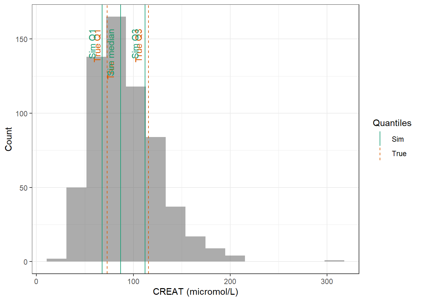
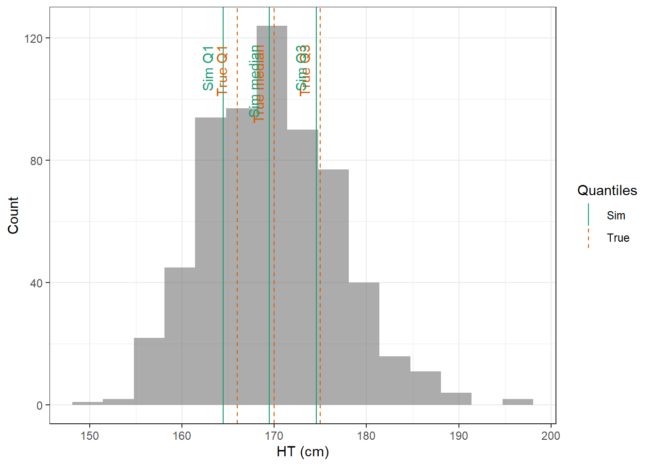
evaluate_cov_sim <- function(p, q, cov_name, cov_unit, cov_sim) {
  #' Plot simulated covariate distribution versus observed quantiles from the paper
  #' @param p numeric vector of probabilities
  #' @param q numeric vector of quantiles
  #' @param cov_name character string containing the covariate name
  #' @param cov_unit character string containing the unit of the covariate
  #' @param cov_sim tibble containing the simulated values for the covariate
  #' @return ggplot2 showing the distributions of the simulated covariate and the observed covariate quantiles
  
  
  #create a dataset with the true percentiles to be able to show them on the plot
  true_percentiles <- tibble(p, q) |> 
    mutate(label = case_match(p, 
                              0 ~ "True min",
                              0.25 ~ "True Q1",
                              0.5 ~ "True median",
                              0.75 ~ "True Q3",
                              1 ~ "True max")) 
  
  #create a dataset with the percentiles of the fitted distributions to be able to show them on the plot
   sim_percentiles <-  tibble(
    probability = p,
    q = quantile(pull(cov_sim,cov_name),p) 
  ) |> 
        mutate(label = case_match(probability, 
                              0 ~ "Sim min",
                              0.25 ~ "Sim Q1",
                              0.5 ~ "Sim median",
                              0.75 ~ "Sim Q3",
                              1 ~ "Sim max"))
   
# create an initial histogram in order to be able to extract statistics of the binned covariate
hist_ini <- ggplot(cov_sim, aes(x = .data[[cov_name]])) +
  geom_histogram(bins=15)
   
hist_data <- layer_data(hist_ini)
   
plot <- ggplot(hist_data) +
  geom_rect(aes(xmin=xmin,xmax=xmax, ymin=0, ymax=count),
            alpha = 0.5) +
     geom_vline(data = true_percentiles,
                mapping = aes(xintercept = q,color = "True"),
                lty = "dashed") +
     geom_vline(data = sim_percentiles,
                mapping = aes(xintercept = q,color = "Sim"),
                lty = "solid") +
     theme_bw() +
     ylab("Count") +
     xlab(paste0(cov_name, " (", cov_unit, ")"))  +

     geom_text(
       data = true_percentiles,
       mapping = aes(x = q, label = label, color = "True"),
       show.legend = FALSE,
       y = 0.95*max(hist_data$ymax),
       hjust = 1,
       vjust = -1,
       angle = 90
     ) +
     geom_text(
       data = sim_percentiles,
       mapping = aes(x = q, label = label, color = "Sim"),
       show.legend = FALSE,
       y = 0.95*max(hist_data$ymax),
       hjust = 1,
       vjust = -1,
       angle = 90
     ) +
     scale_color_brewer(name = "Quantiles",
                        palette ="Dark2")
   plot
}

plot_sim_cov_wrapper <- function(cov_data,cov_name,cov_sim){
  cov_df <- extract_cov_param(cov_data, cov_name)

evaluate_cov_sim(cov_df$p,cov_df$q,cov_df$cov_name,cov_df$cov_unit,
                 cov_sim)
}

plot_sim_cov_wrapper(cov_data_carlier,"CRCL",sim_cov_carlier)

plot_sim_cov_wrapper(cov_data_carlier,"WT",sim_cov_carlier)

plot_sim_cov_wrapper(cov_data_carlier,"AGE",sim_cov_carlier)

plot_sim_cov_wrapper(cov_data_carlier,"BMI",sim_cov_carlier)

Then, based on BMI and WT, height (HT) is calculated to be able to calculate the body surface area (BSA). CRCL was calculated using the measured urinary equation, and as we have know information about the urinary volume or urinary creatinine concentration, we cannot reconvert CRCL to CREAT based on this equation. The most recommended equation is CKD-EPI, however as different exponents are used based on the value of CREAT, it can’t be used for reconversion of CRCL to CREAT. Thus, the second best equation, MDRD is used.

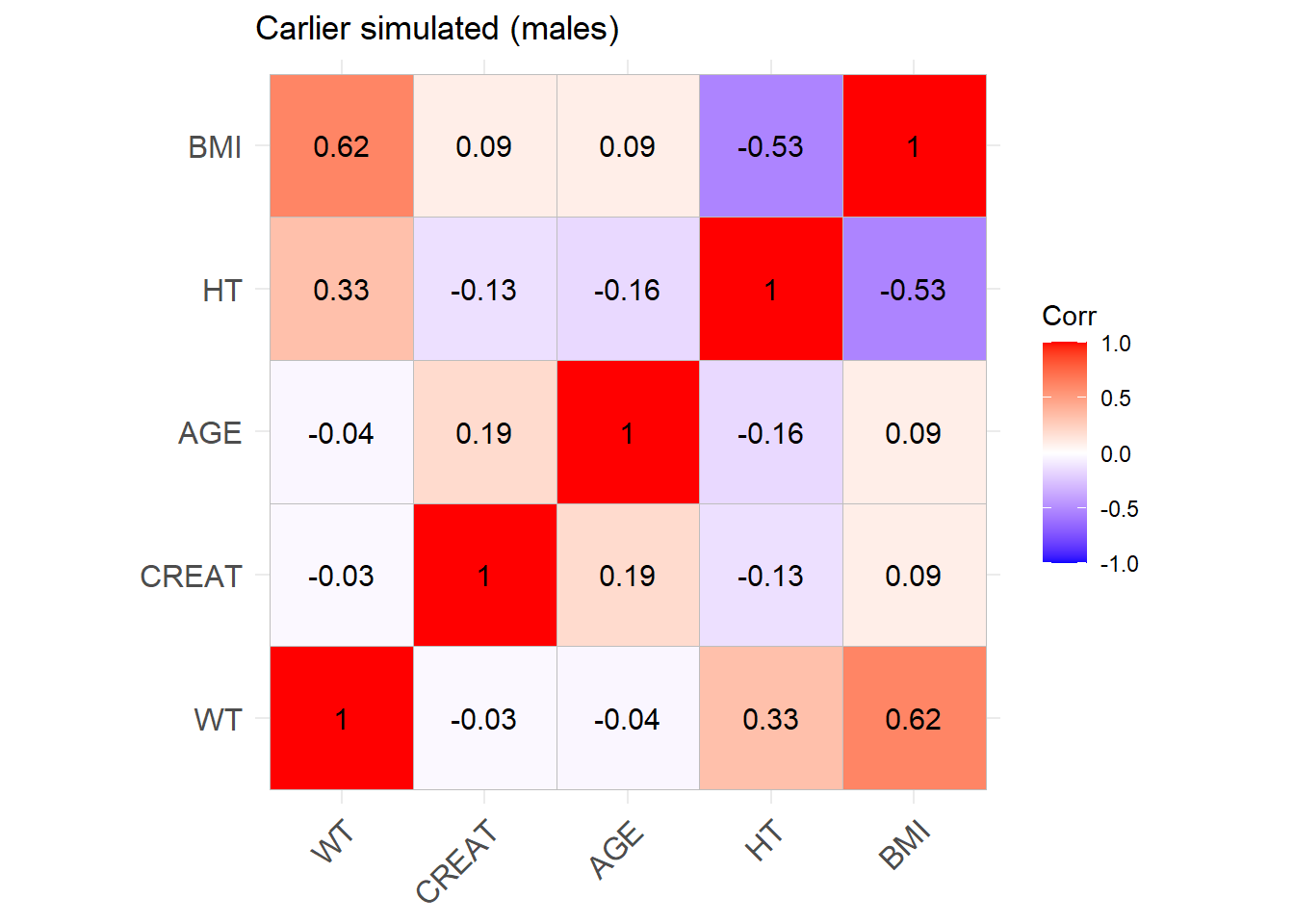
reconvert_MDRD <- function(AGE, CRCL, SEX) {
    # Mutliply by 0.742 for females
    sex_factor <- ifelse(SEX == 0, 1, 0.742)
    
    # Calculate DFG
   CREAT <- (CRCL / (175 * (AGE^(-0.203)) * sex_factor))^(-1 / 1.154)
  
  return(CREAT)
}

sim_cov_carlier <- sim_cov_carlier %>%
  mutate(
    BSA = (WT^0.425 * (HT^0.725) * 0.007184), # Calculate body surface area based on Dubois&Dubois formula
    CRCL = CRCL * (1.73 /BSA) # convert mL/min to mL/min/1.73 m2
  )
sim_cov_carlier$CREAT <- mapply(reconvert_MDRD, sim_cov_carlier$AGE, sim_cov_carlier$CRCL, sim_cov_carlier$SEX)
sim_cov_carlier <- sim_cov_carlier %>%
  dplyr::select(Paper, ID_within_paper, ICU, BURN, OBESE, CREAT, WT, BSA, BMI, AGE, SEX, HT)

# Calculate the simulated correlation matrices separately for the two sexes to compare with the original
sim_cov_carlier_M <- sim_cov_carlier %>% filter(SEX == 0)
sim_cov_carlier_F <- sim_cov_carlier %>% filter(SEX == 1)

cor_sim_M <- cor(sim_cov_carlier_M %>% dplyr::select(WT, CREAT, AGE, HT, BMI), use = "complete.obs")
cor_sim_F <- cor(sim_cov_carlier_F %>% dplyr::select(WT, CREAT, AGE, HT, BMI), use = "complete.obs")

ggcorrplot(cor_matrix_Carlier_F, lab = TRUE, title = "Carlier original (females)")

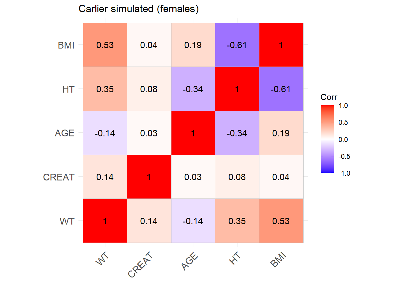
Carlier_F <- ggcorrplot(cor_sim_F, lab = TRUE, title = "Carlier simulated (females)")
Carlier_F 

ggcorrplot(cor_matrix_Carlier_M, lab = TRUE, title = "Carlier original (males)")

Carlier_M <- ggcorrplot(cor_sim_M, lab = TRUE, title = "Carlier simulated (males)")
Carlier_M

5.3 Fournier et al. (2018)

5.4 General considerations about the paper

This study includes only 21 patients, thus deriving distributions from the reported covariates values might be difficult

5.4.1 Covariate distribution

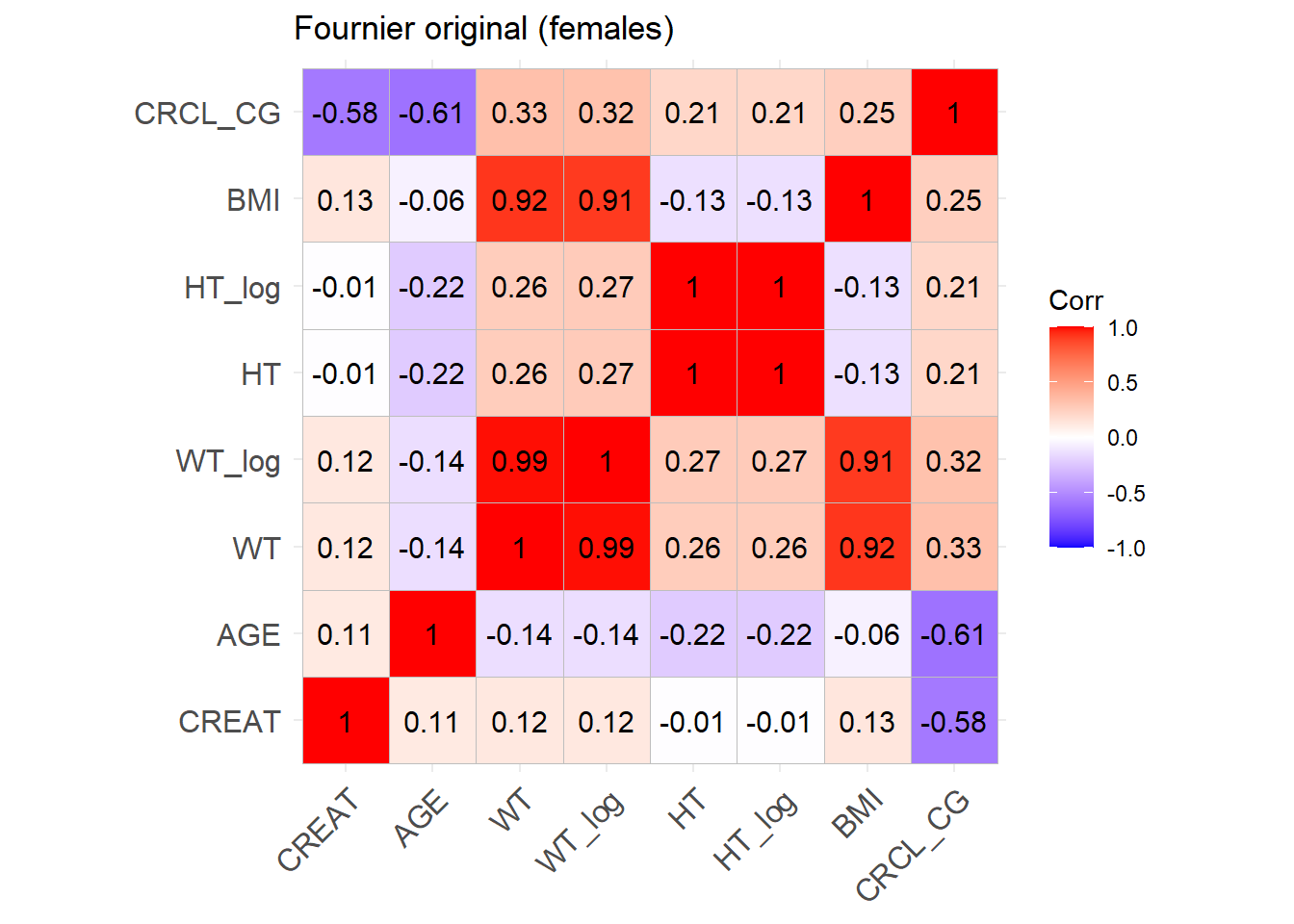
All patients are ICU patients with burns who are assumed to be non obese. Creatinine clearance is calculated based on the Cockcroft & Gault equation, whose output is in mL/min, so there is no need to calculate BSA. Thus for all patients ICU = 1, BURN = 1 and OBESE=0.

It is not mentioned in the article if certain patients are on renal replacement therapy, therefore we assume that they are not, and set the minimum value of creatinine clearance to 10 mL/min. CRCL was estimated using the Cockroft and Gault equation.

For AGE, not the median and IQR is given but the mean (50.1) and standard deviation (24.3). As we cannot compare the simulated distribution to the true one, so we suppose that the distribution follows a normal distribution.

The proportion of males in the original article is 0.762.

Neither BMI nor HT or BSA are provided in the article, thus the height is simulated based on the height obtained from the MIMIC clinical dataset (normal distribution with mean of 169 and sd of 10.3).

For WT, AGE and CRCL here are the data from the paper :

cov_data_fournier <- cov_data |> 
  filter(Paper == "Fournier_2018")

cov_data_fournier |> 
  filter(Covariate %in% c("WT","CRCL","AGE")) |> 
  kable()

Paper	Covariate	Unit	Median	Q1	Q3	Min	Max
Fournier_2018	WT	kg	72.4	67	83.6	NA	NA
Fournier_2018	CRCL	mL/min	128.0	65	150.0	10	NA
Fournier_2018	AGE	year	50.1	NA	NA	NA	NA

cor_matrix_Fournier_F <- readRDS(here("Simulations/cor_matrix_Fournier_F.rds"))
print(cor_matrix_Fournier_F)

              CREAT         AGE         WT     WT_log          HT      HT_log
CREAT    1.00000000  0.11092068  0.1240980  0.1236777 -0.01115272 -0.01163038
AGE      0.11092068  1.00000000 -0.1411092 -0.1377268 -0.21810675 -0.21757157
WT       0.12409798 -0.14110923  1.0000000  0.9910295  0.26291857  0.26261857
WT_log   0.12367767 -0.13772678  0.9910295  1.0000000  0.27210890  0.27214801
HT      -0.01115272 -0.21810675  0.2629186  0.2721089  1.00000000  0.99936169
HT_log  -0.01163038 -0.21757157  0.2626186  0.2721480  0.99936169  1.00000000
BMI      0.13219801 -0.06085883  0.9199729  0.9108563 -0.12595561 -0.12641807
CRCL_CG -0.57789581 -0.60548019  0.3271195  0.3230419  0.20870474  0.20811864
                BMI    CRCL_CG
CREAT    0.13219801 -0.5778958
AGE     -0.06085883 -0.6054802
WT       0.91997291  0.3271195
WT_log   0.91085635  0.3230419
HT      -0.12595561  0.2087047
HT_log  -0.12641807  0.2081186
BMI      1.00000000  0.2518084
CRCL_CG  0.25180837  1.0000000

ggcorrplot(cor_matrix_Fournier_F, lab = TRUE, title = "Sex: female")

cor_matrix_Fournier_M <- readRDS(here("Simulations/cor_matrix_Fournier_M.rds"))
print(cor_matrix_Fournier_M)

              CREAT         AGE          WT      WT_log          HT      HT_log
CREAT    1.00000000  0.08421679  0.07887415  0.07757763 -0.01796103 -0.01782471
AGE      0.08421679  1.00000000 -0.11683417 -0.11039865 -0.13268497 -0.13114182
WT       0.07887415 -0.11683417  1.00000000  0.99316445  0.36730646  0.36578272
WT_log   0.07757763 -0.11039865  0.99316445  1.00000000  0.36989373  0.36884368
HT      -0.01796103 -0.13268497  0.36730646  0.36989373  1.00000000  0.99929302
HT_log  -0.01782471 -0.13114182  0.36578272  0.36884368  0.99929302  1.00000000
BMI      0.09421423 -0.05819520  0.87199105  0.86717872 -0.12604976 -0.12807159
CRCL_CG -0.60813562 -0.55803721  0.29302773  0.28921272  0.18756329  0.18568377
                BMI    CRCL_CG
CREAT    0.09421423 -0.6081356
AGE     -0.05819520 -0.5580372
WT       0.87199105  0.2930277
WT_log   0.86717872  0.2892127
HT      -0.12604976  0.1875633
HT_log  -0.12807159  0.1856838
BMI      1.00000000  0.2145950
CRCL_CG  0.21459503  1.0000000

ggcorrplot(cor_matrix_Fournier_M, lab = TRUE, title = "Sex: male")

fournier_crcl <- fit_cov_wrapper(
  cov_data = cov_data_fournier,
  cov_name = "CRCL",
  min_plot = 0,
  max_plot = 250,
  tol=0.002
)

fournier_crcl$plot

Tolerance was increased to 0.002 to have a fit for log-normal. Normal distribution is better suited.

fournier_wt <- fit_cov_wrapper(
  cov_data = cov_data_fournier,
  cov_name = "WT",
  min_plot = 40,
  max_plot = 120
)

fournier_wt$plot

In this case the log-normal distribution quantiles are closer to the true quantiles than the normal ones. We will take the log-normal ones.

5.4.2 Simulation of covariates

Covariates will be sampled from the following distributions :

• CRCL : Normal distribution with mean 117.016 mL/min and standard deviation 63.3 mL/min
• WT : Lognormal distribution with mean 73.8 kg, and coefficient of variation 17 %
• AGE : Supposed normal distribution with mean of 50.1 years and standard deviation of 24.3

The proportion of males is 0.762 in the original article, so the number of males is 476 and the number of females is 149 to add up to 625.

correlated_simulation <- function(n, means, cov_matrix) {
  set.seed(1991)
  collected <- matrix(NA, 0, length(means))
  colnames(collected) <- names(means)

  while (nrow(collected) < n) {
    batch <- MASS::mvrnorm(n = n, mu = means, Sigma = cov_matrix)
    colnames(batch) <- names(means)

    valid <- batch[, "AGE"] >= 18 &
             batch[, "CRCL_CG"] >= 10

    batch_valid <- batch[valid, , drop = FALSE]
    collected <- rbind(collected, batch_valid)
  }

  collected[1:n, , drop = FALSE]
}

means <- c(
  CRCL_CG = fournier_crcl$norm_par["mean"],
  WT_log      = fournier_wt$lnorm_par["meanlog"],
  AGE     = 50.1,
  HT = 169
)

sds <- c(
  CRCL_CG = fournier_crcl$norm_par["sd"],
  WT_log      = fournier_wt$lnorm_par["sdlog"],
  AGE     = 24.3,
  HT = 10.3
)

covariates <- c("CRCL_CG", "WT_log", "AGE", "HT")

names(means) <- covariates

# Correlation and Covariance Matrix
cor_fournier_M <- cor_matrix_Fournier_M[covariates, covariates]
cov_matrix_M <- diag(sds) %*% cor_fournier_M %*% diag(sds)
eigen(cov_matrix_M)$values

[1] 4218.3820076  387.0322287  102.1295861    0.0230053

cor_fournier_F <- cor_matrix_Fournier_F[covariates, covariates]
cov_matrix_F <- diag(sds) %*% cor_fournier_F %*% diag(sds)
eigen(cov_matrix_F)$values

[1] 4.253434e+03 3.545807e+02 9.952763e+01 2.398513e-02

# Simulate
sim_data_M <- correlated_simulation(n = 476, means = means, cov_matrix = cov_matrix_M)
sim_data_M <- as_tibble(sim_data_M) %>%
  mutate(SEX = 0)

sim_data_F <- correlated_simulation(n = 149, means = means, cov_matrix = cov_matrix_F)
sim_data_F <- as_tibble(sim_data_F) %>%
  mutate(SEX = 1)

sim_data <- rbind(sim_data_M, sim_data_F)

# Put the covariates together
sim_cov_fournier <- tibble(
  Paper = "Fournier_2018",
  ID_within_paper = 1:n_patient,
  ICU = 1,
  BURN = 1,
  OBESE = 0,
  CRCL = sim_data$CRCL_CG,
  WT_log   = sim_data$WT_log,
  AGE  = sim_data$AGE,
  HT  = sim_data$HT,
  SEX = sim_data$SEX)

sim_cov_fournier <- sim_cov_fournier %>%
  mutate(WT = exp(WT_log))

summary_sim_cov_fournier <- sim_cov_fournier |> 
  pivot_longer(cols = c(ICU,BURN,OBESE,CRCL,WT,AGE),
               names_to = "Covariate") |> 
  summarise(.by = c(Covariate,Paper),
            Min = min(value),
            Q1 = quantile(value, 0.25),
            Median = quantile(value, 0.5),
            Q3 = quantile(value, 0.75),
            Max = max(value))

paste0("The proportion of males is ", round(mean(sim_cov_fournier$SEX == 0), 3), " compared to the original 0.762.")

[1] "The proportion of males is 0.762 compared to the original 0.762."

cov_fournier_compare <- summary_sim_cov_fournier |>
  rename_with(~ paste0(.x, "_sim"), -one_of("Covariate", "Paper")) |>
  left_join(rename_with(
    cov_data_fournier,
    ~ paste0(.x, "_true"),
    -one_of("Covariate", "Paper", "Unit")
  )) |> 
  relocate(Covariate, .after = Paper) |> 
  relocate(Unit, .after = Covariate)

cov_fournier_compare |>
  gt() |>
  fmt_scientific() |> 
    tab_spanner(columns = starts_with("Min"),
              label = "Min") |> 
      tab_spanner(columns = starts_with("Q1"),
              label = "Q1") |> 
      tab_spanner(columns = starts_with("Median"),
              label = "Median") |> 
      tab_spanner(columns = starts_with("Q3"),
              label = "Q3") |> 
  tab_spanner(columns = starts_with("Max"),
              label = "Max")

Paper	Covariate	Unit	Min		Q1		Median		Q3		Max
			Min_sim	Min_true	Q1_sim	Q1_true	Median_sim	Median_true	Q3_sim	Q3_true	Max_sim	Max_true
Fournier_2018	ICU	Unitless	1.00	1.00	1.00	1.00	1.00	1.00	1.00	1.00	1.00	1.00
Fournier_2018	BURN	Unitless	1.00	1.00	1.00	1.00	1.00	1.00	1.00	1.00	1.00	1.00
Fournier_2018	OBESE	Unitless	0.00	0.00	0.00	0.00	0.00	0.00	0.00	0.00	0.00	0.00
Fournier_2018	CRCL	mL/min	1.01 × 101	1.00 × 101	7.32 × 101	6.50 × 101	1.16 × 102	1.28 × 102	1.55 × 102	1.50 × 102	2.88 × 102	NA
Fournier_2018	WT	kg	4.53 × 101	NA	6.66 × 101	6.70 × 101	7.45 × 101	7.24 × 101	8.40 × 101	8.36 × 101	1.18 × 102	NA
Fournier_2018	AGE	year	1.80 × 101	NA	3.49 × 101	NA	5.03 × 101	5.01 × 101	6.72 × 101	NA	1.31 × 102	NA

plot_sim_cov_wrapper(cov_data_fournier,"CRCL",sim_cov_fournier)

plot_sim_cov_wrapper(cov_data_fournier,"WT",sim_cov_fournier)

plot_sim_cov_wrapper(cov_data_fournier,"AGE",sim_cov_fournier)

Then, based on the BMI and WT, the height (HT) is calculated to be able to calculate the body surface area (BSA). CRCL is reconverted to serum creatinine (CREAT) based on the Cockroft and Gault equation.

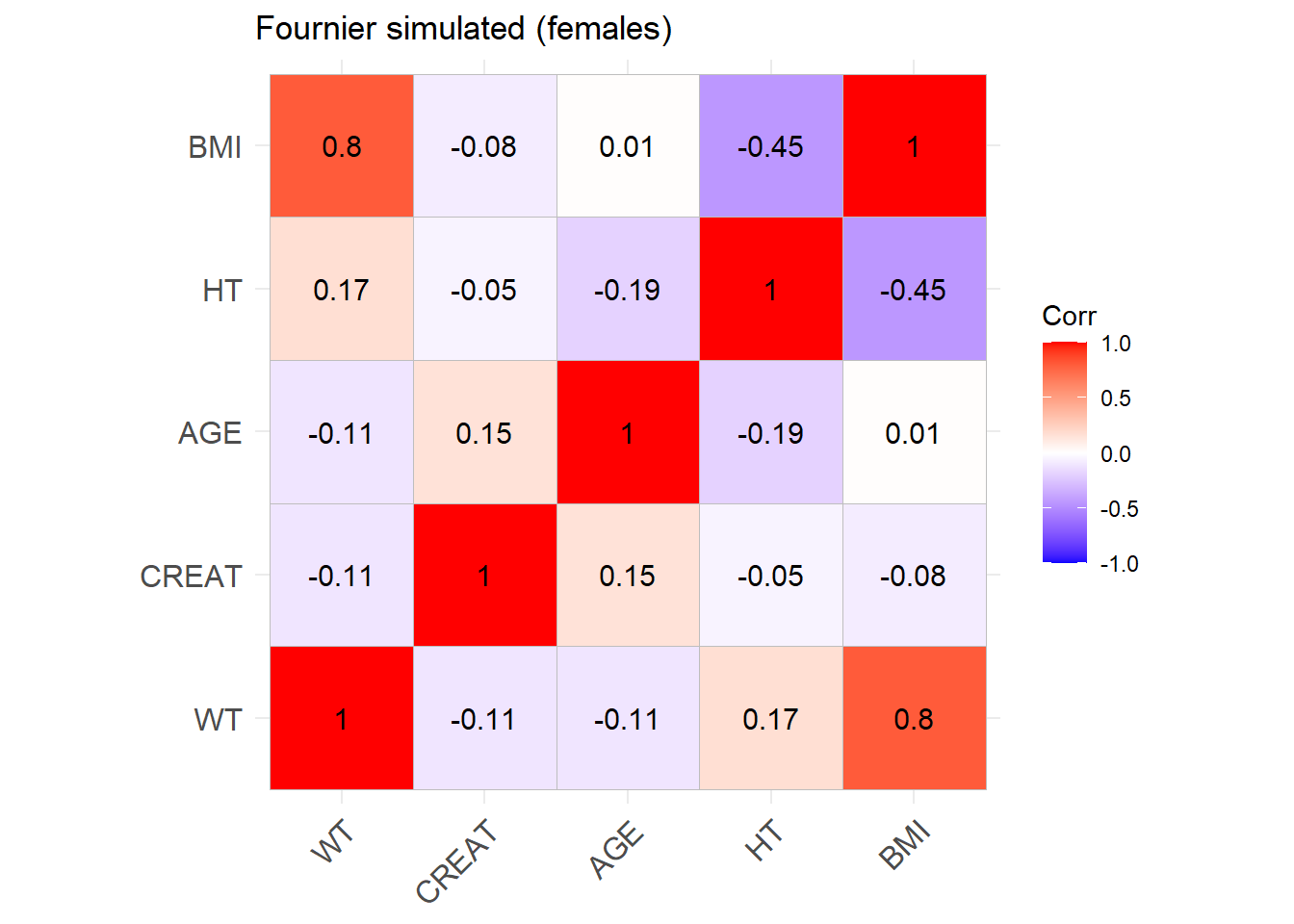
reconvert_CG <- function(AGE, CRCL, SEX, WT) {
    # Mutliply by 0.85 for females
    sex_factor <- ifelse(SEX == 0, 1, 0.85)
    
    # Calculate DFG
    CREAT = ((140 - AGE) * WT * sex_factor) / (CRCL * 72)
  
  return(CREAT)
}

sim_cov_fournier$CREAT <- mapply(reconvert_CG, sim_cov_fournier$AGE, sim_cov_fournier$CRCL, sim_cov_fournier$SEX, sim_cov_fournier$WT)
sim_cov_fournier <- sim_cov_fournier %>%
  mutate(
     BSA = (WT^0.425 * (HT^0.725) * 0.007184),
     BMI = WT / (HT/100)^2,
     OBESE = ifelse(BMI > 30, 1, 0)
  ) %>%
  dplyr::select(Paper, ID_within_paper, ICU, BURN, OBESE, CREAT, WT, BSA, BMI, AGE, SEX, HT)
# Calculate the simulated correlation matrices separately for the two sexes to compare with the original
sim_cov_fournier_M <- sim_cov_fournier %>% filter(SEX == 0)
sim_cov_fournier_F <- sim_cov_fournier %>% filter(SEX == 1)

cor_sim_M <- cor(sim_cov_fournier_M %>% dplyr::select(WT, CREAT, AGE, HT, BMI), use = "complete.obs")
cor_sim_F <- cor(sim_cov_fournier_F %>% dplyr::select(WT, CREAT, AGE, HT, BMI), use = "complete.obs")

ggcorrplot(cor_matrix_Fournier_F, lab = TRUE, title = "Fournier original (females)")

Fournier_F <- ggcorrplot(cor_sim_F, lab = TRUE, title = "Fournier simulated (females)")
Fournier_F

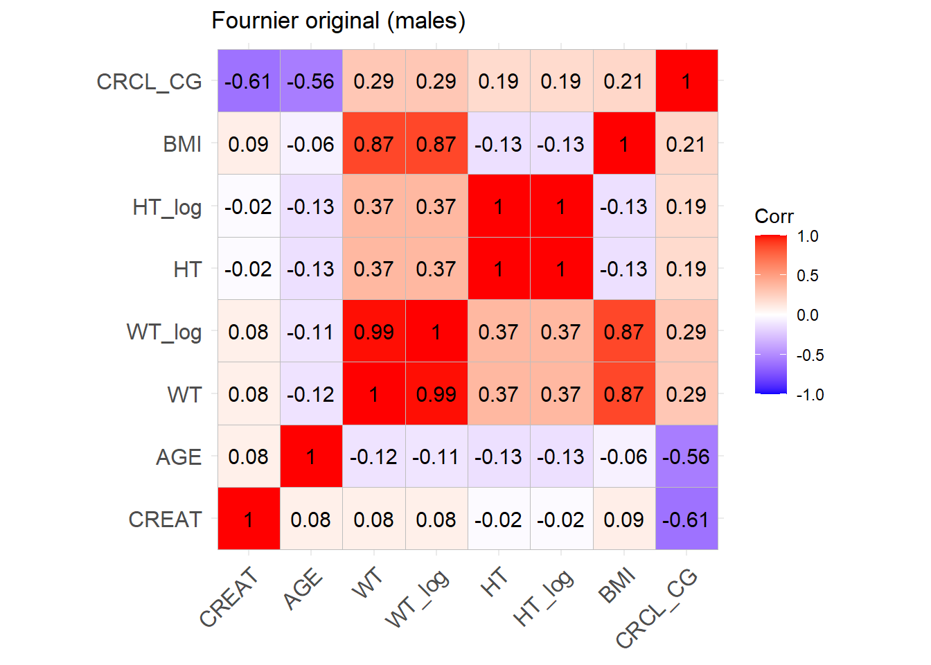
ggcorrplot(cor_matrix_Fournier_M, lab = TRUE, title = "Fournier original (males)")

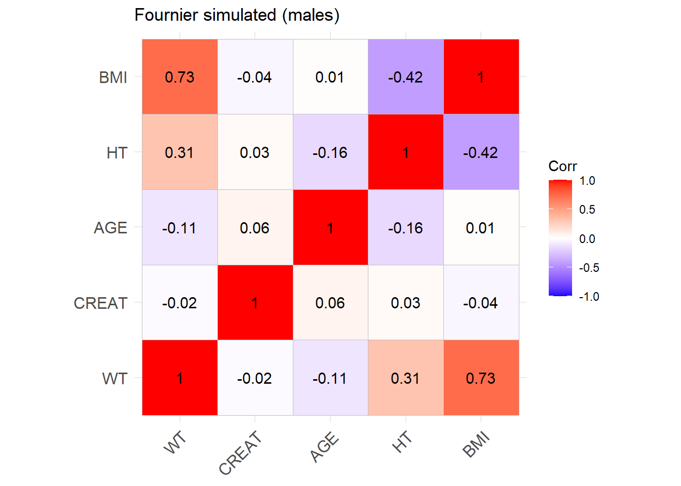
Fournier_M <- ggcorrplot(cor_sim_M, lab = TRUE, title = "Fournier simulated (males)")
Fournier_M

5.5 Mellon et al. (2020)

5.5.1 Covariate distribution

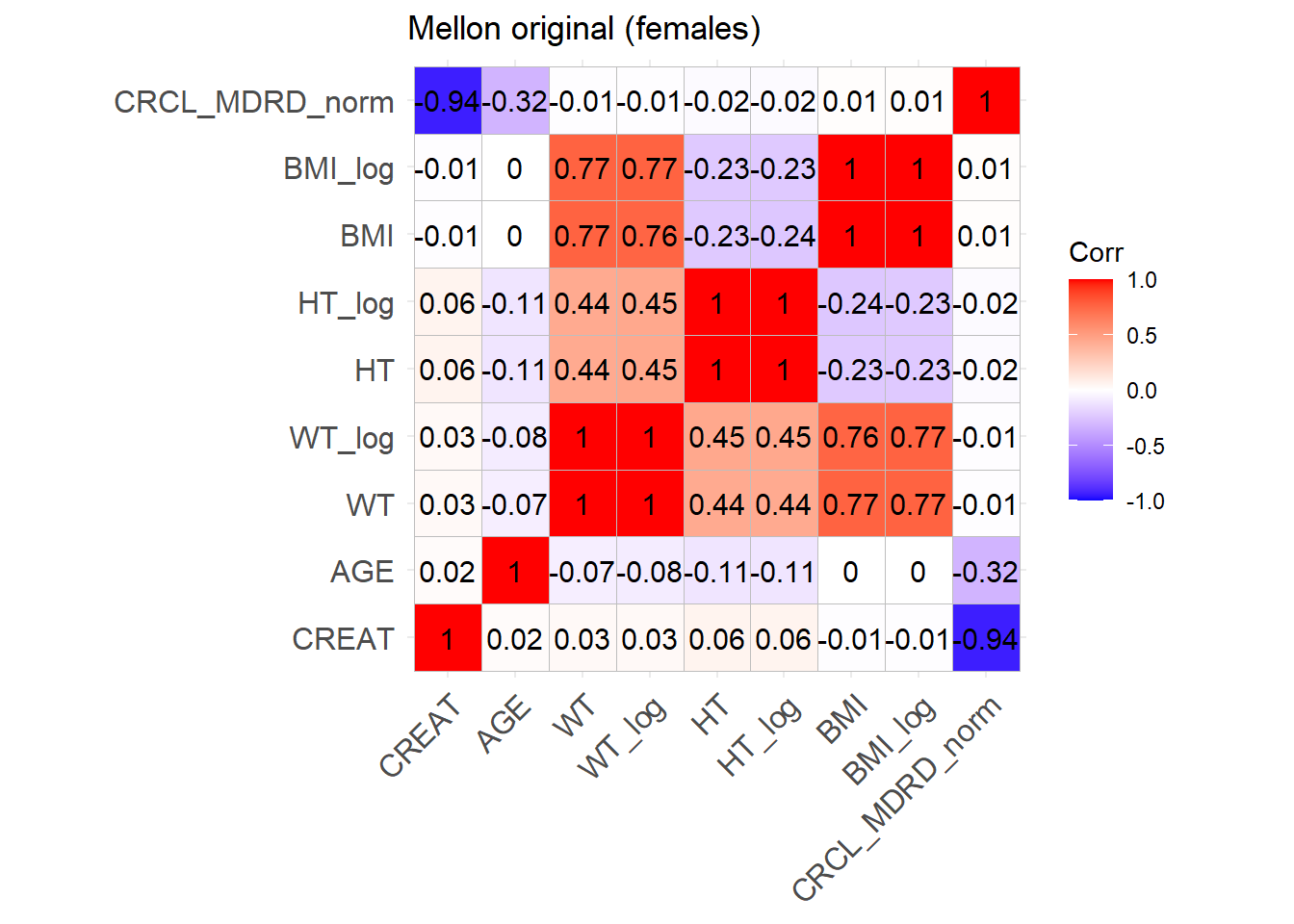
Patients are obese, but otherwise healthy, meaning that they are not in intensive care and not burn victims. They are all obese (BMI > 30 kg/m^2). Creatinine clearance is calculated based on the MDRD equation. Thus for all patients ICU = 0, BURN = 0, OBESE=1.

For WT, BMI and CRCL here are the data from the paper :

cov_data_mellon <- cov_data |> 
  filter(Paper == "Mellon_2020")

cov_data_mellon |> 
  filter(Covariate %in% c("WT","CRCL", "AGE", "BMI", "BMI_log")) |> 
  kable()

Paper	Covariate	Unit	Median	Q1	Q3	Min	Max
Mellon_2020	WT	kg	109.3	NA	NA	88.00	151.50
Mellon_2020	CRCL	mL/min/1.73m^{2}	94.0	NA	NA	62.00	133.00
Mellon_2020	BMI	kg/m^{2}	40.6	NA	NA	35.20	67.30
Mellon_2020	BMI_log	kg/m^{2}	3.7	NA	NA	3.56	4.21
Mellon_2020	CRCL	ml/min	NA	NA	NA	NA	NA
Mellon_2020	AGE	year	51.7	NA	NA	22.90	62.90

cor_matrix_Mellon_F <- readRDS(here("Simulations/cor_matrix_Mellon_F.rds"))
print(cor_matrix_Mellon_F)

                      CREAT          AGE          WT       WT_log          HT
CREAT           1.000000000  0.022643469  0.03125540  0.031968067  0.05795702
AGE             0.022643469  1.000000000 -0.07488881 -0.077065515 -0.11168121
WT              0.031255400 -0.074888809  1.00000000  0.997431167  0.43988528
WT_log          0.031968067 -0.077065515  0.99743117  1.000000000  0.45364368
HT              0.057957020 -0.111681207  0.43988528  0.453643683  1.00000000
HT_log          0.057716460 -0.110775924  0.43501172  0.448949779  0.99935506
BMI            -0.006435320 -0.004011043  0.76869713  0.758978914 -0.23142245
BMI_log        -0.006781559 -0.004085614  0.77244329  0.765197692 -0.22615779
CRCL_MDRD_norm -0.936664533 -0.319596180 -0.00640208 -0.006556334 -0.02317188
                    HT_log          BMI      BMI_log CRCL_MDRD_norm
CREAT           0.05771646 -0.006435320 -0.006781559   -0.936664533
AGE            -0.11077592 -0.004011043 -0.004085614   -0.319596180
WT              0.43501172  0.768697132  0.772443287   -0.006402080
WT_log          0.44894978  0.758978914  0.765197692   -0.006556334
HT              0.99935506 -0.231422452 -0.226157792   -0.023171879
HT_log          1.00000000 -0.237225021 -0.231732528   -0.023241184
BMI            -0.23722502  1.000000000  0.997187131    0.009471973
BMI_log        -0.23173253  0.997187131  1.000000000    0.009607333
CRCL_MDRD_norm -0.02324118  0.009471973  0.009607333    1.000000000

ggcorrplot(cor_matrix_Mellon_F, lab = TRUE, title = "Sex: female")

cor_matrix_Mellon_M <- readRDS(here("Simulations/cor_matrix_Mellon_M.rds"))
print(cor_matrix_Mellon_M)

                      CREAT          AGE           WT       WT_log           HT
CREAT           1.000000000 -0.079420098 -0.005155970 -0.002021643  0.062039693
AGE            -0.079420098  1.000000000 -0.020403922 -0.018224696 -0.002835067
WT             -0.005155970 -0.020403922  1.000000000  0.997694029  0.617330996
WT_log         -0.002021643 -0.018224696  0.997694029  1.000000000  0.634363996
HT              0.062039693 -0.002835067  0.617330996  0.634363996  1.000000000
HT_log          0.061429587 -0.001756480  0.613093576  0.631018266  0.999227265
BMI            -0.070072797 -0.019345942  0.535836189  0.518641232 -0.328796339
BMI_log        -0.069673338 -0.020297428  0.545596150  0.528796578 -0.319827206
CRCL_MDRD_norm -0.940158336 -0.215895006  0.007018922  0.003387753 -0.059982333
                    HT_log         BMI     BMI_log CRCL_MDRD_norm
CREAT           0.06142959 -0.07007280 -0.06967334   -0.940158336
AGE            -0.00175648 -0.01934594 -0.02029743   -0.215895006
WT              0.61309358  0.53583619  0.54559615    0.007018922
WT_log          0.63101827  0.51864123  0.52879658    0.003387753
HT              0.99922726 -0.32879634 -0.31982721   -0.059982333
HT_log          1.00000000 -0.33401211 -0.32475168   -0.059647213
BMI            -0.33401211  1.00000000  0.99775044    0.069173500
BMI_log        -0.32475168  0.99775044  1.00000000    0.069388818
CRCL_MDRD_norm -0.05964721  0.06917350  0.06938882    1.000000000

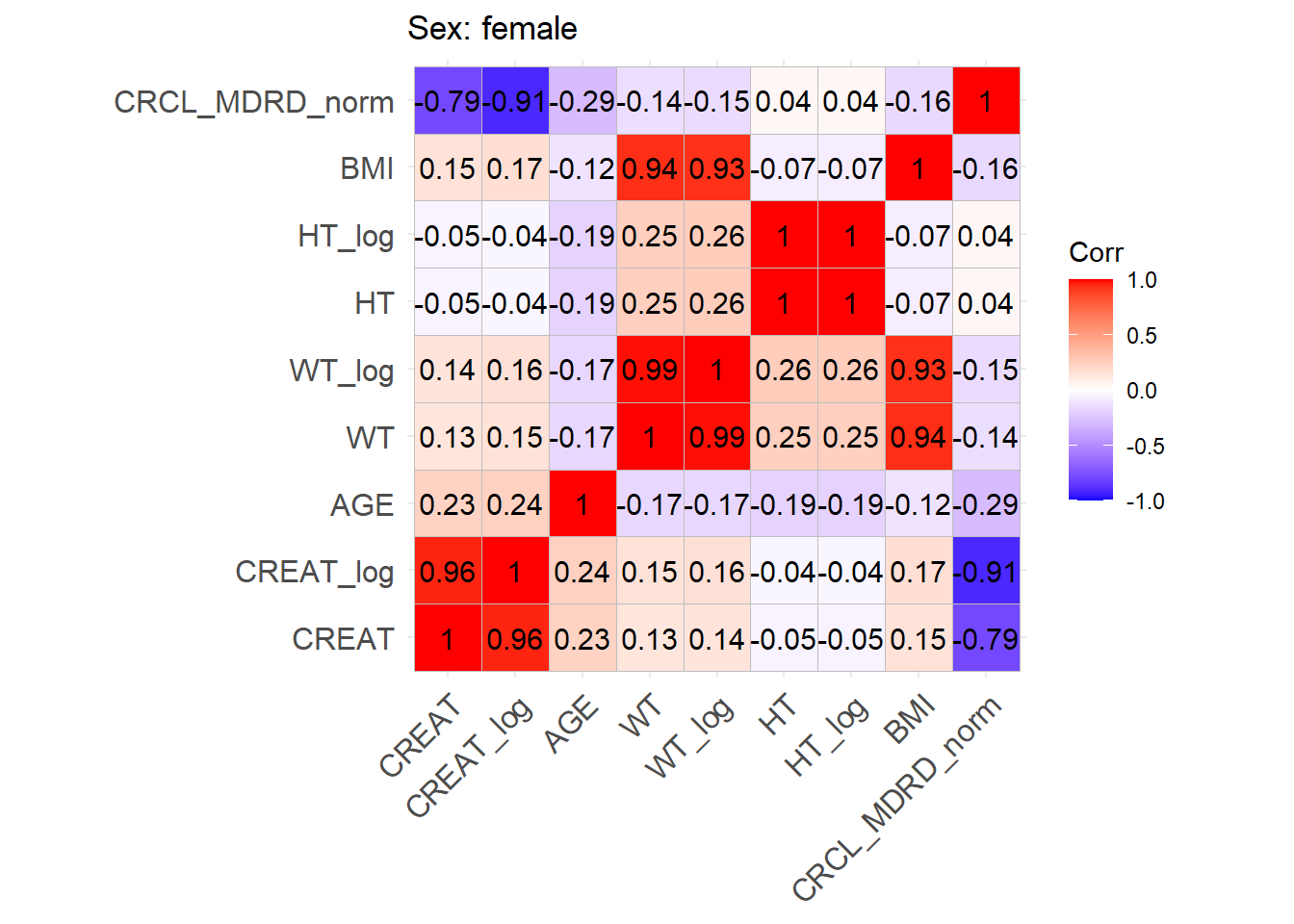
ggcorrplot(cor_matrix_Mellon_M, lab = TRUE, title = "Sex: male")

Mellon is different from the other papers as CRCL is given as ml/min/1.73m^{2} based on the MDRD equation, and instead of Q1 and Q3, the minimum and maxiumum of the covariates is given (apart from BMI). Another particularity is that due to the particularity of the subjects (obesity), the distribution of body weight is positively (right) skewed. Positively skewed distribution is relatively rare, so it is not easy to find a distribution function to describe it. Beta distribution needs scaling the data between 0 and 1. and 4 parameter stable distribution et gamma distribution have several parameters that need to be defined, and in the absence of the original data, it is not possible to estimate these parameters.

The proportion of males is 0.148.

mellon_crcl <- fit_cov_wrapper(
  cov_data = cov_data_mellon,
  cov_name = "CRCL",
  min_plot = 0,
  max_plot = 250
)

mellon_crcl$plot

Similar fits; normal distribution is selected.

mellon_wt <- fit_cov_wrapper(
  cov_data = cov_data_mellon,
  cov_name = "WT",
  min_plot = 40,
  max_plot = 170
)

mellon_wt$plot

Log-normal distribution fits slightly better than normal.

mellon_age <- fit_cov_wrapper(
  cov_data = cov_data_mellon,
  cov_name = "AGE",
  min_plot = 0,
  max_plot = 120
)

mellon_age$plot

Normal distribution fits a bit better.

mellon_bmi <- fit_cov_wrapper(
  cov_data = cov_data_mellon,
  cov_name = "BMI",
  min_plot = 0,
  max_plot = 100, 
  tol = 0.001
)

mellon_bmi$plot

mellon_bmi_log <- fit_cov_wrapper(
  cov_data = cov_data_mellon,
  cov_name = "BMI_log",
  min_plot = 2.5,
  max_plot = 5, 
  tol = 0.001
)

mellon_bmi_log$plot

Log-normal distribution fits a bit better.

5.5.2 Simulation of covariates

Covariates will be sampled from the following distributions :

• CRCL : Normal distribution from which negative values have been resampled, with mean 94 mL/min and standard deviation 14.3 mL/min
• WT : Log-normal distribution with mean 109 kg, and coefficient of variation 9.41 %
• AGE : Normal distribution with mean 2.84^{22} years, and standard deviation 4.81 %
• BMI : Log-normal distribution with mean 40.6 \(kg/m^{2}\), and coefficient of variation 6.14 %

The proportion of males is 0.148 in the original article, so the number of males is 93 and the number of females is 532 to add up to 625.

correlated_simulation <- function(n, means, cov_matrix) {
  set.seed(1991)
  collected <- matrix(NA, 0, length(means))
  colnames(collected) <- names(means)

  while (nrow(collected) < n) {
    batch <- MASS::mvrnorm(n = n, mu = means, Sigma = cov_matrix)
    colnames(batch) <- names(means)

    valid <- batch[, "AGE"] >= 18 &
             batch[, "CRCL_MDRD_norm"] >= 10 &
             batch[, "BMI_log"] > 3.401197 # log(30)

    batch_valid <- batch[valid, , drop = FALSE]
    collected <- rbind(collected, batch_valid)
  }

  collected[1:n, , drop = FALSE]
}

means <- c(
  CRCL_MDRD_norm = mellon_crcl$norm_par["mean"],
  WT_log      = mellon_wt$lnorm_par["meanlog"],
  AGE     = mellon_age$norm_par["mean"],
  BMI_log     = mellon_bmi$lnorm_par["meanlog"]
)

sds <- c(
  CRCL_MDRD_norm = mellon_crcl$norm_par["sd"],
  WT_log      = mellon_wt$lnorm_par["sdlog"], 
  AGE = mellon_age$norm_par["sd"],
  BMI_log     = mellon_bmi$lnorm_par["sdlog"]
)

covariates <- c("CRCL_MDRD_norm", "WT_log", "AGE", "BMI_log")

names(means) <- covariates

# Correlation and Covariance Matrix
cor_mellon_M <- cor_matrix_Mellon_M[covariates, covariates]
cov_matrix_M <- diag(sds) %*% cor_mellon_M %*% diag(sds)
eigen(cov_matrix_M)$values

[1] 2.050769e+02 2.197051e+01 1.024041e-02 2.320348e-03

cor_mellon_F <- cor_matrix_Mellon_F[covariates, covariates]
cov_matrix_F <- diag(sds) %*% cor_mellon_F %*% diag(sds)
eigen(cov_matrix_F)$values

[1] 2.064991e+02 2.054837e+01 1.132511e-02 1.194553e-03

# Simulate
sim_data_M <- correlated_simulation(n = 93, means = means, cov_matrix = cov_matrix_M)
sim_data_M <- as_tibble(sim_data_M) %>%
  mutate(SEX = 0)

sim_data_F <- correlated_simulation(n = 532, means = means, cov_matrix = cov_matrix_F)
sim_data_F <- as_tibble(sim_data_F) %>%
  mutate(SEX = 1)

sim_data <- rbind(sim_data_M, sim_data_F)

# Put the covariates together
sim_cov_mellon <- tibble(
  Paper = "Mellon_2020",
  ID_within_paper = 1:n_patient,
  ICU = 0,
  BURN = 0,
  OBESE = 1,
  CRCL = sim_data$CRCL_MDRD_norm,
  WT_log   = sim_data$WT_log,
  AGE  = sim_data$AGE,
  BMI_log  = sim_data$BMI_log,
  SEX = sim_data$SEX)

sim_cov_mellon <- sim_cov_mellon %>%
  mutate(WT = exp(WT_log),
         BMI = exp(BMI_log))

summary_sim_cov_mellon <- sim_cov_mellon |> 
  pivot_longer(cols = c(ICU,BURN,OBESE,CRCL,WT,AGE),
               names_to = "Covariate") |> 
  summarise(.by = c(Covariate,Paper),
            Min = min(value),
            Q1 = quantile(value, 0.25),
            Median = quantile(value, 0.5),
            Q3 = quantile(value, 0.75),
            Max = max(value))

sim_cov_mellon <- sim_cov_mellon %>%
  dplyr::select(Paper, ID_within_paper, ICU, BURN, OBESE, CRCL, WT, AGE, BMI, SEX)

cov_mellon_compare <- summary_sim_cov_mellon |>
  rename_with(~ paste0(.x, "_sim"), -one_of("Covariate", "Paper")) |>
  left_join(rename_with(
    cov_data_mellon,
    ~ paste0(.x, "_true"),
    -one_of("Covariate", "Paper", "Unit")
  )) |> 
  relocate(Covariate, .after = Paper) |> 
  relocate(Unit, .after = Covariate)

cov_mellon_compare |>
  gt() |>
  fmt_scientific() |> 
  tab_spanner(columns = starts_with("Min"),
              label = "Min") |> 
  tab_spanner(columns = starts_with("Q1"),
              label = "Q1") |> 
  tab_spanner(columns = starts_with("Median"),
              label = "Median") |> 
  tab_spanner(columns = starts_with("Q3"),
              label = "Q3") |> 
  tab_spanner(columns = starts_with("Max"),
              label = "Max")

Paper	Covariate	Unit	Min		Q1		Median		Q3		Max
			Min_sim	Min_true	Q1_sim	Q1_true	Median_sim	Median_true	Q3_sim	Q3_true	Max_sim	Max_true
Mellon_2020	ICU	Unitless	0.00	0.00	0.00	0.00	0.00	0.00	0.00	0.00	0.00	0.00
Mellon_2020	BURN	Unitless	0.00	0.00	0.00	0.00	0.00	0.00	0.00	0.00	0.00	0.00
Mellon_2020	OBESE	Unitless	1.00	1.00	1.00	1.00	1.00	1.00	1.00	1.00	1.00	1.00
Mellon_2020	CRCL	mL/min/1.73m^{2}	5.18 × 101	6.20 × 101	8.24 × 101	NA	9.39 × 101	9.40 × 101	1.05 × 102	NA	1.48 × 102	1.33 × 102
Mellon_2020	CRCL	ml/min	5.18 × 101	NA	8.24 × 101	NA	9.39 × 101	NA	1.05 × 102	NA	1.48 × 102	NA
Mellon_2020	WT	kg	8.10 × 101	8.80 × 101	1.02 × 102	NA	1.09 × 102	1.09 × 102	1.16 × 102	NA	1.41 × 102	1.51 × 102
Mellon_2020	AGE	year	3.51 × 101	2.29 × 101	4.87 × 101	NA	5.22 × 101	5.17 × 101	5.57 × 101	NA	7.07 × 101	6.29 × 101

Then, based on the BMI and WT, the height (HT) is calculated to be able to calculate the body surface area (BSA). CRCL is reconverted to serum creatinine (CREAT) based on the MDRD equation.

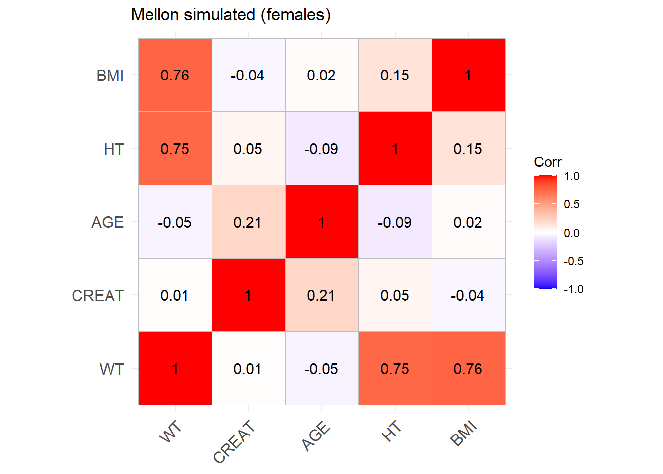
reconvert_MDRD <- function(AGE, CRCL, SEX) {
    # Mutliply by 0.85 for females
    sex_factor <- ifelse(SEX == 0, 1, 0.742)
    
    # Calculate DFG
   CREAT <- (CRCL / (175 * (AGE^(-0.203)) * sex_factor))^(-1 / 1.154)
  
  return(CREAT)
}

sim_cov_mellon$CREAT <- mapply(reconvert_MDRD, sim_cov_mellon$AGE, sim_cov_mellon$CRCL, sim_cov_mellon$SEX)
sim_cov_mellon <- sim_cov_mellon %>%
  mutate(
   HT = sqrt(WT/BMI) * 100, # mutliplied by 100 to convert m to cm
    BSA = (WT^0.425 * (HT^0.725) * 0.007184),
    OBESE = ifelse(BMI > 30, 1, 0)
  ) %>%
  dplyr::select(Paper, ID_within_paper, ICU, BURN, OBESE, CREAT, WT, BSA, BMI, AGE, SEX, HT)

# Calculate the simulated correlation matrices separately for the two sexes to compare with the original
sim_cov_mellon_M <- sim_cov_mellon %>% filter(SEX == 0)
sim_cov_mellon_F <- sim_cov_mellon %>% filter(SEX == 1)

cor_sim_M <- cor(sim_cov_mellon_M %>% dplyr::select(WT, CREAT, AGE, HT, BMI), use = "complete.obs")
cor_sim_F <- cor(sim_cov_mellon_F %>% dplyr::select(WT, CREAT, AGE, HT, BMI), use = "complete.obs")

ggcorrplot(cor_matrix_Mellon_F, lab = TRUE, title = "Mellon original (females)")

Mellon_F <- ggcorrplot(cor_sim_F, lab = TRUE, title = "Mellon simulated (females)")
Mellon_F

ggcorrplot(cor_matrix_Mellon_M, lab = TRUE, title = "Mellon original (males)")

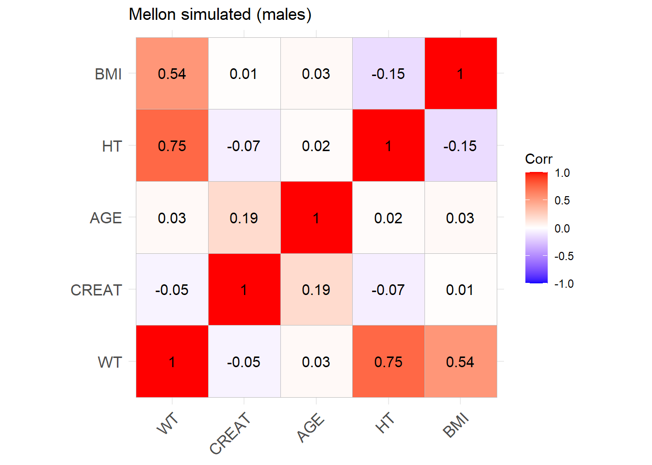
Mellon_M <- ggcorrplot(cor_sim_M, lab = TRUE, title = "Mellon simulated (males)")
Mellon_M

5.6 Rambaud et al. (2020)

5.6.1 Covariate distribution

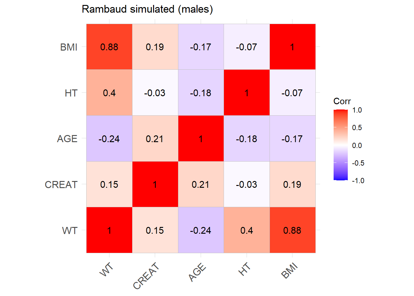
All patients are ICU patients with endocarditis. They are not considered to be burn victims or obese. Creatinine clearance was calculated using the CKD-EPI equation. Thus for all patients ICU = 1, BURN = 0 and OBESE=0. In this paper, the distribution of serum creatinine is given (in micromol/L), so it can be directly simulated instead of reconverting CRCL. The proportion of males is 0.794.

For WT and CRCL here are the data from the paper :

cov_data_rambaud <- cov_data |> 
  filter(Paper == "Rambaud_2020")

cov_data_rambaud |> 
  filter(Covariate %in% c("WT","CREAT","AGE","HT")) |> 
  kable()

Paper	Covariate	Unit	Median	Q1	Q3	Min	Max
Rambaud_2020	WT	kg	76	69	87.0	NA	NA
Rambaud_2020	HT	cm	170	166	175.0	NA	NA
Rambaud_2020	AGE	year	72	62	80.5	NA	NA
Rambaud_2020	CREAT	micromol/L	87	73	115.5	NA	NA

cor_matrix_Rambaud_F <- readRDS(here("Simulations/cor_matrix_Rambaud_F.rds"))
print(cor_matrix_Rambaud_F)

                     CREAT   CREAT_log        AGE         WT     WT_log
CREAT           1.00000000  0.96241769  0.2320510  0.1329905  0.1360852
CREAT_log       0.96241769  1.00000000  0.2429180  0.1521950  0.1565402
AGE             0.23205099  0.24291801  1.0000000 -0.1726236 -0.1683232
WT              0.13299046  0.15219495 -0.1726236  1.0000000  0.9894565
WT_log          0.13608520  0.15654017 -0.1683232  0.9894565  1.0000000
HT             -0.04892509 -0.04044581 -0.1889338  0.2517176  0.2592944
HT_log         -0.04916482 -0.04082750 -0.1894298  0.2520660  0.2599500
BMI             0.15464517  0.17128168 -0.1162404  0.9435277  0.9336719
CRCL_MDRD_norm -0.78792478 -0.91391033 -0.2872002 -0.1410118 -0.1466372
                        HT      HT_log        BMI CRCL_MDRD_norm
CREAT          -0.04892509 -0.04916482  0.1546452    -0.78792478
CREAT_log      -0.04044581 -0.04082750  0.1712817    -0.91391033
AGE            -0.18893375 -0.18942976 -0.1162404    -0.28720016
WT              0.25171756  0.25206601  0.9435277    -0.14101184
WT_log          0.25929441  0.25994996  0.9336719    -0.14663719
HT              1.00000000  0.99970438 -0.0747791     0.04109155
HT_log          0.99970438  1.00000000 -0.0742787     0.04153856
BMI            -0.07477910 -0.07427870  1.0000000    -0.15925725
CRCL_MDRD_norm  0.04109155  0.04153856 -0.1592572     1.00000000

ggcorrplot(cor_matrix_Rambaud_F, lab = TRUE, title = "Sex: female")

cor_matrix_Rambaud_M <- readRDS(here("Simulations/cor_matrix_Rambaud_M.rds"))
print(cor_matrix_Rambaud_M)

                      CREAT     CREAT_log        AGE          WT      WT_log
CREAT           1.000000000  0.9686820232  0.1909639  0.09370644  0.09181062
CREAT_log       0.968682023  1.0000000000  0.1982311  0.12356685  0.12378068
AGE             0.190963871  0.1982311079  1.0000000 -0.18051719 -0.17233815
WT              0.093706437  0.1235668470 -0.1805172  1.00000000  0.99225399
WT_log          0.091810623  0.1237806818 -0.1723382  0.99225399  1.00000000
HT             -0.005710820  0.0007327162 -0.1229902  0.37551772  0.37978066
HT_log         -0.005537361  0.0010029509 -0.1228308  0.37500256  0.37967684
BMI             0.103837382  0.1331126943 -0.1347419  0.89436959  0.88815355
CRCL_MDRD_norm -0.769174641 -0.8857730397 -0.2449519 -0.12508733 -0.12881176
                          HT       HT_log         BMI CRCL_MDRD_norm
CREAT          -0.0057108200 -0.005537361  0.10383738   -0.769174641
CREAT_log       0.0007327162  0.001002951  0.13311269   -0.885773040
AGE            -0.1229902101 -0.122830828 -0.13474194   -0.244951935
WT              0.3755177211  0.375002564  0.89436959   -0.125087326
WT_log          0.3797806561  0.379676845  0.88815355   -0.128811758
HT              1.0000000000  0.999598212 -0.07118055   -0.003915605
HT_log          0.9995982117  1.000000000 -0.07162513   -0.004244813
BMI            -0.0711805452 -0.071625134  1.00000000   -0.133475436
CRCL_MDRD_norm -0.0039156049 -0.004244813 -0.13347544    1.000000000

ggcorrplot(cor_matrix_Rambaud_M, lab = TRUE, title = "Sex: male")

rambaud_creat <- fit_cov_wrapper(
  cov_data = cov_data_rambaud,
  cov_name = "CREAT",
  min_plot = 0,
  max_plot = 250
)

rambaud_creat$plot

Log-normal distribution fits the best the data, so it is selected.

rambaud_wt <- fit_cov_wrapper(
  cov_data = cov_data_rambaud,
  cov_name = "WT",
  min_plot = 40,
  max_plot = 120
)

rambaud_wt$plot

No discernable difference between the two fits. The log-normal distribution is selected.

rambaud_age <- fit_cov_wrapper(
  cov_data = cov_data_rambaud,
  cov_name = "AGE",
  min_plot = 0,
  max_plot = 120
)

rambaud_age$plot

No discernable difference, so normal distribution is selected, as age usually follows a normal distribution.

rambaud_ht <- fit_cov_wrapper(
  cov_data = cov_data_rambaud,
  cov_name = "HT",
  min_plot = 140,
  max_plot = 200
)

rambaud_ht$plot

No discernable difference. Log-normal distribution is selected.

5.6.2 Simulation of covariates

Covariates will be sampled from the following distributions :

• CREAT : Log-normal distribution with a minimum 10 micromol/L with mean 89.7 micromol/L and standard deviation 0.346 micromol/L
• WT : Normal distribution with resampling of negative values with mean 76.8 kg, and standard deviation 17.3 %
• AGE : Normal distribution with resampling of negative values with mean 1.22^{31} years, and coefficient of variation 1370 %
• HT : Normal distribution with resampling of negative values with mean 170 cm, and standard deviation 3.93 %

The proportion of males is 0.794 in the original article, so the number of males is 496 and the number of females is 129 to add up to 625.

correlated_simulation <- function(n, means, cov_matrix) {
  set.seed(1991)
  collected <- matrix(NA, 0, length(means))
  colnames(collected) <- names(means)

  while (nrow(collected) < n) {
    batch <- MASS::mvrnorm(n = n, mu = means, Sigma = cov_matrix)
    colnames(batch) <- names(means)

    valid <- batch[, "AGE"] >= 18 &
             batch[, "CREAT_log"] < 5.991465 # log(400) corresponding to CRCL of 10 mL/min for a patient of 24 kg and 116 years

    batch_valid <- batch[valid, , drop = FALSE]
    collected <- rbind(collected, batch_valid)
  }

  collected[1:n, , drop = FALSE]
}

means <- c(
  CREAT_log = rambaud_creat$lnorm_par["meanlog"],
  WT_log      = rambaud_wt$lnorm_par["meanlog"], 
  AGE     = rambaud_age$norm_par["mean"],
  HT_log      = rambaud_ht$lnorm_par["meanlog"]
)

sds <- c(
  CREAT_log = rambaud_creat$lnorm_par["sdlog"],
  WT_log     = rambaud_wt$lnorm_par["sdlog"],
  AGE = rambaud_age$norm_par["sd"],
  HT_log     = rambaud_ht$lnorm_par["sdlog"]
)

covariates <- c("CREAT_log", "WT_log", "AGE", "HT_log")

names(means) <- covariates

# Correlation and Covariance Matrix
cor_rambaud_M <- cor_matrix_Rambaud_M[covariates, covariates]
cov_matrix_M <- diag(sds) %*% cor_rambaud_M %*% diag(sds)
eigen(cov_matrix_M)$values

[1] 1.888441e+02 1.160604e-01 2.831560e-02 1.302147e-03

cor_rambaud_F <- cor_matrix_Rambaud_F[covariates, covariates]
cov_matrix_F <- diag(sds) %*% cor_rambaud_F %*% diag(sds)
eigen(cov_matrix_F)$values

[1] 1.888465e+02 1.143105e-01 2.761902e-02 1.396003e-03

# Simulate
sim_data_M <- correlated_simulation(n = 496, means = means, cov_matrix = cov_matrix_M)
sim_data_M <- as_tibble(sim_data_M) %>%
  mutate(SEX = 0)

sim_data_F <- correlated_simulation(n = 129, means = means, cov_matrix = cov_matrix_F)
sim_data_F <- as_tibble(sim_data_F) %>%
  mutate(SEX = 1)

sim_data <- rbind(sim_data_M, sim_data_F)

# Put the covariates together
sim_cov_rambaud <- tibble(
  Paper = "Rambaud_2020",
  ID_within_paper = 1:n_patient,
  ICU = 1,
  BURN = 0,
  OBESE = 0,
  CREAT_log = sim_data$CREAT_log,
  WT_log   = sim_data$WT_log,
  AGE  = sim_data$AGE,
  HT_log  = sim_data$HT_log,
  SEX = sim_data$SEX)

sim_cov_rambaud <- sim_cov_rambaud %>%
  mutate(CREAT = exp(CREAT_log),
         HT = exp(HT_log),
         WT = exp(WT_log))

summary_sim_cov_rambaud <- sim_cov_rambaud |> 
  pivot_longer(cols = c(ICU,BURN,OBESE,CREAT,WT,AGE,HT),
               names_to = "Covariate") |> 
  summarise(.by = c(Covariate,Paper),
            Min = min(value),
            Q1 = quantile(value, 0.25),
            Median = quantile(value, 0.5),
            Q3 = quantile(value, 0.75),
            Max = max(value))

cov_rambaud_compare <- summary_sim_cov_rambaud |>
  rename_with(~ paste0(.x, "_sim"), -one_of("Covariate", "Paper")) |>
  left_join(rename_with(
    cov_data_rambaud,
    ~ paste0(.x, "_true"),
    -one_of("Covariate", "Paper", "Unit")
  )) |> 
  relocate(Covariate, .after = Paper) |> 
  relocate(Unit, .after = Covariate)

cov_rambaud_compare |>
  gt() |>
  fmt_scientific() |> 
    tab_spanner(columns = starts_with("Min"),
              label = "Min") |> 
      tab_spanner(columns = starts_with("Q1"),
              label = "Q1") |> 
      tab_spanner(columns = starts_with("Median"),
              label = "Median") |> 
      tab_spanner(columns = starts_with("Q3"),
              label = "Q3") |> 
  tab_spanner(columns = starts_with("Max"),
              label = "Max")

Paper	Covariate	Unit	Min		Q1		Median		Q3		Max
			Min_sim	Min_true	Q1_sim	Q1_true	Median_sim	Median_true	Q3_sim	Q3_true	Max_sim	Max_true
Rambaud_2020	ICU	Unitless	1.00	1.00	1.00	1.00	1.00	1.00	1.00	1.00	1.00	1.00
Rambaud_2020	BURN	Unitless	0.00	0.00	0.00	0.00	0.00	0.00	0.00	0.00	0.00	0.00
Rambaud_2020	OBESE	Unitless	0.00	0.00	0.00	0.00	0.00	0.00	0.00	0.00	0.00	0.00
Rambaud_2020	CREAT	micromol/L	2.08 × 101	NA	6.79 × 101	7.30 × 101	8.67 × 101	8.70 × 101	1.12 × 102	1.15 × 102	3.08 × 102	NA
Rambaud_2020	WT	kg	4.13 × 101	NA	6.75 × 101	6.90 × 101	7.65 × 101	7.60 × 101	8.64 × 101	8.70 × 101	1.21 × 102	NA
Rambaud_2020	AGE	year	1.97 × 101	NA	6.04 × 101	6.20 × 101	7.08 × 101	7.20 × 101	8.20 × 101	8.05 × 101	1.12 × 102	NA
Rambaud_2020	HT	cm	1.50 × 102	NA	1.64 × 102	1.66 × 102	1.69 × 102	1.70 × 102	1.75 × 102	1.75 × 102	1.96 × 102	NA

plot_sim_cov_wrapper(cov_data_rambaud,"CREAT",sim_cov_rambaud)

plot_sim_cov_wrapper(cov_data_rambaud,"WT",sim_cov_rambaud)

plot_sim_cov_wrapper(cov_data_rambaud,"AGE",sim_cov_rambaud)

plot_sim_cov_wrapper(cov_data_rambaud,"HT",sim_cov_rambaud)

CREAT is converted from micromol/L to mg/dL.

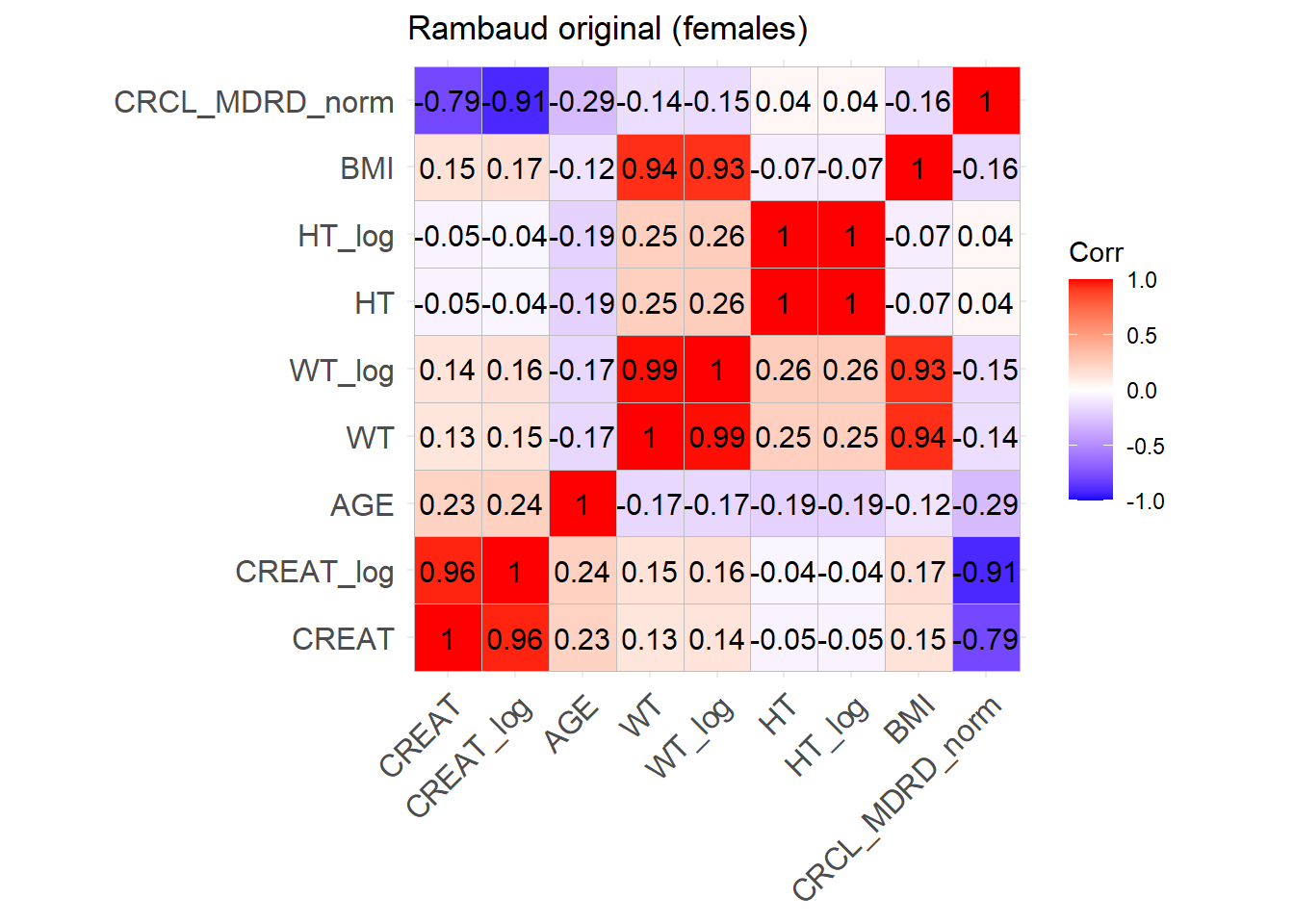
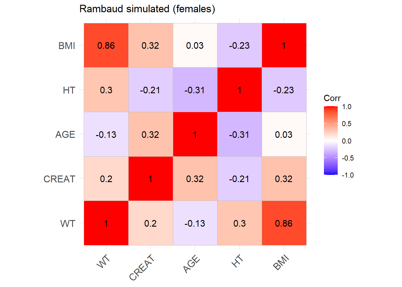
sim_cov_rambaud <- sim_cov_rambaud %>%
  mutate(
    BSA = (WT^0.425 * (HT^0.725) * 0.007184),
    CREAT = CREAT/88.4,
    BMI = WT / (HT/100)^2,
    OBESE = ifelse(BMI > 30, 1, 0)
  ) %>%
  dplyr::select(Paper, ID_within_paper, ICU, BURN, OBESE, CREAT, WT, BSA, BMI, AGE, SEX, HT)

# Calculate the simulated correlation matrices separately for the two sexes to compare with the original
sim_cov_rambaud_M <- sim_cov_rambaud %>% filter(SEX == 0)
sim_cov_rambaud_F <- sim_cov_rambaud %>% filter(SEX == 1)

cor_sim_M <- cor(sim_cov_rambaud_M %>% dplyr::select(WT, CREAT, AGE, HT, BMI), use = "complete.obs")
cor_sim_F <- cor(sim_cov_rambaud_F %>% dplyr::select(WT, CREAT, AGE, HT, BMI), use = "complete.obs")

ggcorrplot(cor_matrix_Rambaud_F, lab = TRUE, title = "Rambaud original (females)")

Rambaud_F <- ggcorrplot(cor_sim_F, lab = TRUE, title = "Rambaud simulated (females)")
Rambaud_F

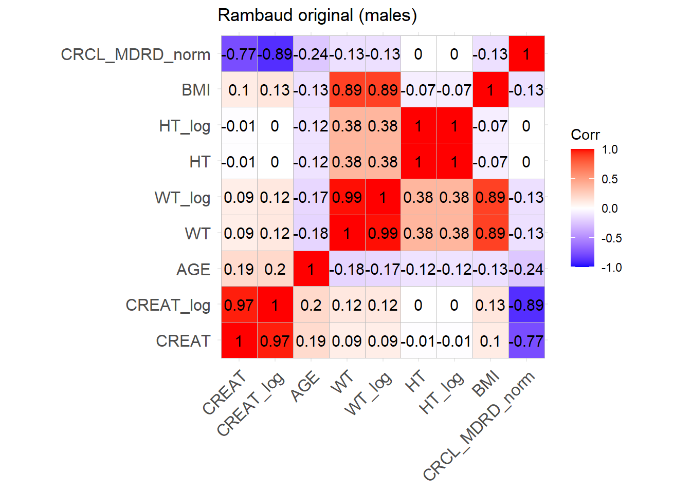
ggcorrplot(cor_matrix_Rambaud_M, lab = TRUE, title = "Rambaud original (males)")

Rambaud_M <- ggcorrplot(cor_sim_M, lab = TRUE, title = "Rambaud simulated (males)")
Rambaud_M

5.7 Final covariate table

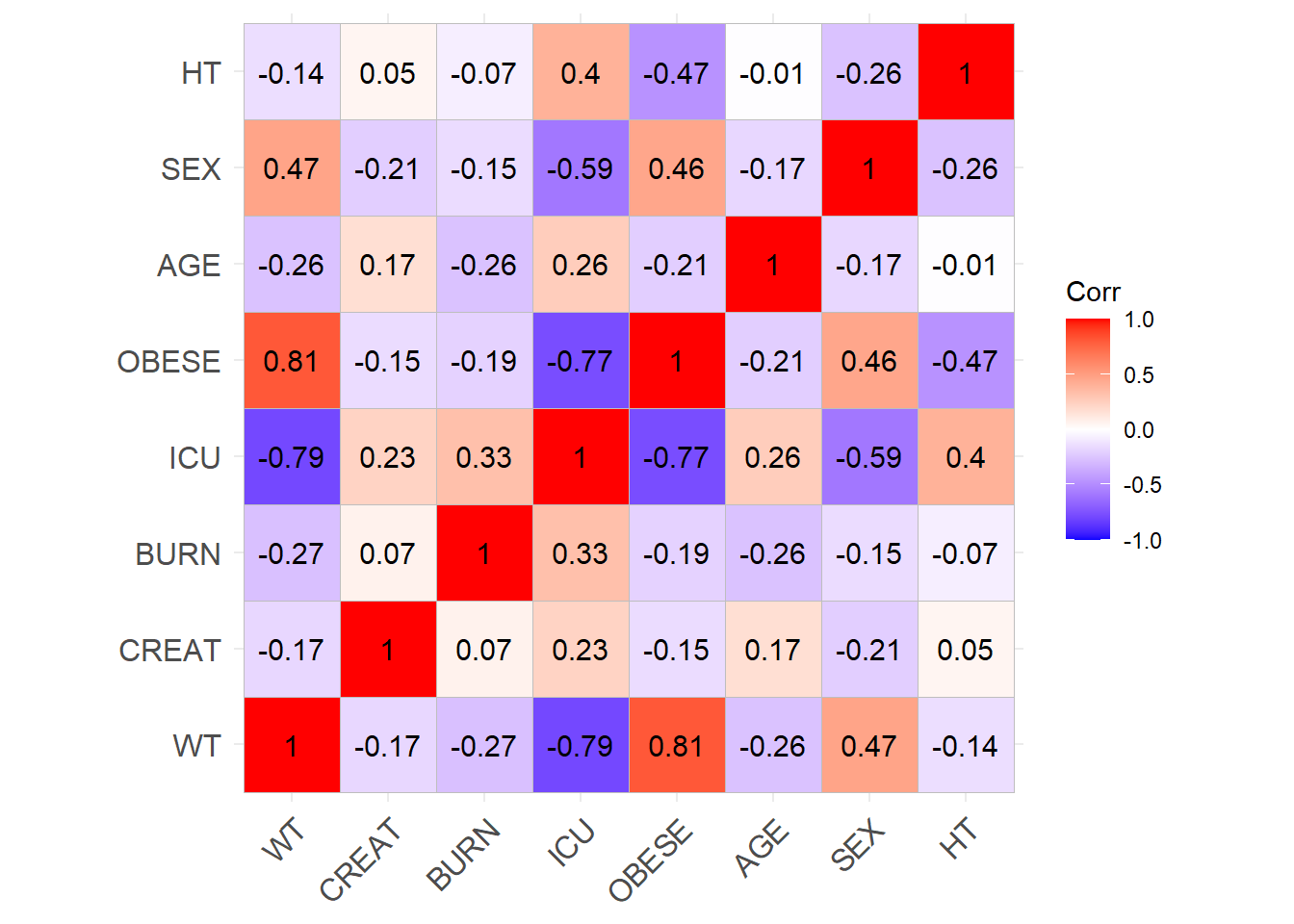
Make the final covariate dataset with 2500 sets of covariates in a way that in each 100 sets, we have 25-25 from each covariate’s cohort, as later, each dosing regimen will be simulated for 100 sets of covariates, and it is important that the 4 cohorts are equally represented.

Also, for the concentration simulation part, we have to know before applying the models, if a patient needs a different regiment due to his renal failure or not. That is why an additional IR column is added where 1 indicates a renal failure patient who needs a dose adjustement. For Carlier, the MDRD equation is used, and for Fournier, the Cockroft and Gault. For Mellon and Rambaud, all patients have 0 in the IR column, as it is not explicited in the articles that a dose adjustement was applied to renal failure patients.

# Patchwork simulated correlation plots
corr_simulated <- (Carlier_F + Fournier_F + Mellon_F + Rambaud_F +
  Carlier_M + Fournier_M + Mellon_M + Rambaud_M) + 
  plot_layout(ncol = 4, nrow = 2, byrow = TRUE)
ggsave(filename = here("Figures/S5.jpg"),
       plot = corr_simulated,
       width = 14, height = 8, dpi = 300)

# Row-bind the datasets to have 25 subjects from each in a sample of 100
datasets <- list(sim_cov_carlier, sim_cov_fournier, sim_cov_mellon, sim_cov_rambaud)

interleave_rows <- function(datasets, chunk_size) {
  n_chunks <- nrow(datasets[[1]]) / chunk_size
  interleaved <- do.call(rbind, lapply(1:n_chunks, function(i) {
    do.call(rbind, lapply(datasets, function(dataset) {
      dataset[((i - 1) * chunk_size + 1):(i * chunk_size), ]
    }))
  }))
  return(interleaved)
}

COV <- interleave_rows(datasets, chunk_size = 25)

# Convert Paper column to MODEL_COHORT column which indicates the model that is used to simulated the covariates
COV <- COV %>%
  mutate(MODEL_COHORT = case_when(
    Paper == "Carlier_2013" ~ "CARLIER",
    Paper == "Fournier_2018" ~ "FOURNIER",
    Paper == "Mellon_2020" ~ "MELLON",
    Paper == "Rambaud_2020" ~ "RAMBAUD")
  )

# Adding ID
COV$ID <- seq(1:2500)

# CRCL calculation functions
calculate_MDRD <- function(AGE, CREAT, SEX) {
  # Mutliply by 0.742 for females
    sex_factor <- ifelse(SEX == 0, 1, 0.742)
    eGFR <- 175 * (CREAT^(-1.154)) * AGE^(-0.203) * sex_factor
    return(eGFR)
}

calculate_CG <- function(AGE, CREAT, SEX, WT) {
  sex_factor <- ifelse(SEX == 0, 1, 0.85)
  eGFR <- ((140 - AGE) * WT * sex_factor) / (CREAT * 72)
  return(eGFR)
}

# Add 1 for dose adjustement for CRCL < 30 mL/min for Carlier and Fournier
COV <- COV %>%
  rowwise() %>%
  mutate(
    CRCL = case_when(
      MODEL_COHORT == "CARLIER" ~ calculate_MDRD(AGE, CREAT, SEX) * (BSA / 1.73),
      MODEL_COHORT == "FOURNIER" ~ calculate_CG(AGE, CREAT, SEX, WT),
      TRUE ~ NA_real_
    ),
    IR = case_when(
      MODEL_COHORT == "CARLIER" & CRCL < 30 ~ 1,
      MODEL_COHORT == "FOURNIER" & CRCL < 30 ~ 1,
      MODEL_COHORT %in% c("MELLON", "RAMBAUD") ~ 0,
      TRUE ~ 0
    )
  ) %>%
  ungroup()

COV <- COV %>%
  dplyr::select(ID, MODEL_COHORT, WT, CREAT, BURN, ICU, OBESE, BSA, AGE, SEX, HT, IR)

# Export to csv
write.csv(COV, here("Data/COV.csv"), quote = F, row.names = F)

# Check correlation (Pearson)
cor_sim <- cor(COV %>% dplyr::select(WT, CREAT, BURN, ICU, OBESE, AGE, SEX, HT), use = "complete.obs")
ggcorrplot(cor_sim, lab = TRUE)

Carlier, Mieke, Michaël Noë, Jan J De Waele, Veronique Stove, Alain G Verstraete, Jeffrey Lipman, and Jason A Roberts. 2013. “Population Pharmacokinetics and Dosing Simulations of Amoxicillin/Clavulanic Acid in Critically Ill Patients.” J. Antimicrob. Chemother. 68 (11): 2600–2608.

Fournier, Anne, Sylvain Goutelle, Yok-Ai Que, Philippe Eggimann, Olivier Pantet, Farshid Sadeghipour, Pierre Voirol, and Chantal Csajka. 2018. “Population Pharmacokinetic Study of Amoxicillin-Treated Burn Patients Hospitalized at a Swiss Tertiary-Care Center.” Antimicrobial Agents and Chemotherapy 62 (9): e00505–18. https://doi.org/10.1128/AAC.00505-18.

Johnson, Alistair E W, Lucas Bulgarelli, Lu Shen, Alvin Gayles, Ayad Shammout, Steven Horng, Tom J Pollard, et al. 2023. “MIMIC-IV, a Freely Accessible Electronic Health Record Dataset.” Sci. Data 10 (1): 1.

Mellon, G, K Hammas, C Burdet, X Duval, C Carette, N El-Helali, L Massias, F Mentré, S Czernichow, and A -C Crémieux. 2020. “Population Pharmacokinetics and Dosing Simulations of Amoxicillin in Obese Adults Receiving Co-Amoxiclav.” Journal of Antimicrobial Chemotherapy 75 (12): 3611–18. https://doi.org/10.1093/jac/dkaa368.

Rambaud, Antoine, Benjamin Jean Gaborit, Colin Deschanvres, Paul Le Turnier, Raphaël Lecomte, Nathalie Asseray-Madani, Anne-Gaëlle Leroy, et al. 2020. “Development and Validation of a Dosing Nomogram for Amoxicillin in Infective Endocarditis.” The Journal of Antimicrobial Chemotherapy 75 (10): 2941–50. https://doi.org/10.1093/jac/dkaa232.