9 Machine learning dose prediction

Show the code

library(openMIPD)
library(dplyr)
library(ggplot2)
library(here)
library(tidyr)
library(stacks)

The data is preprocessed to have the log-transformed daily dose as target variable which allows to reach the target concentration and the data is stratified based on dosing scheme.

Show the code

# Import or generate training and test data
here::i_am("MIPD/Machine_Learning.qmd")

# Create folder to store published figures
if (!dir.exists(here("Figures"))) {
  dir.create(here("Figures"))
}

AMOX_CMIN_TRAIN <- read.csv(here("Data/AMOX_CMIN_TRAIN.csv"), quote = "")

AMOX_CMIN_TEST <- read.csv(here("Data/AMOX_CMIN_TEST.csv"), quote = "")

# The interdose interval column has to be called II
train <- AMOX_CMIN_TRAIN %>%
  dplyr::filter(REFERENCE == 1) %>%
  mutate(II = FREQ)
  
test <- AMOX_CMIN_TEST %>%
  dplyr::filter(REFERENCE == 1) %>%
  mutate(II = FREQ)

# machine learning function from the package
train_preprocessed <- ml_data_preprocess(data = train, target_variable = "CMIN", target_concentration = 60)
test_preprocessed <- ml_data_preprocess(data = test, target_variable = "CMIN", target_concentration = 60)

Show the code

explore_predictions <- function(data, conc_inf = 40, conc_sup = 80, DOSE_PRED) {
  
  dose_pred_col <- sym(DOSE_PRED)

  # Calculate true dose range and prediction correctness
  data <- data %>%
    mutate(
      DOSE_inf = (conc_inf / CMIN_IND) * DOSE_ADM,
      DOSE_sup = (conc_sup / CMIN_IND) * DOSE_ADM
    ) %>%
    mutate(
      Prediction_correctness = ifelse(
        (!!dose_pred_col >= DOSE_inf & !!dose_pred_col <= DOSE_sup),
        "Correct", "Incorrect"
      )
    ) %>%
    drop_na(Prediction_correctness) %>%
    mutate(
      Dosing = case_when(
        Prediction_correctness == "Correct" ~ "On target",
        !!dose_pred_col < DOSE_inf ~ "Underdosed",
        !!dose_pred_col > DOSE_sup ~ "Overdosed"
      )
    )

  # Proportions of under- and overdosing
  dosing <- data %>%
    count(Dosing) %>%
    mutate(
      Proportion = n / sum(n) * 100,
      Dosing = factor(Dosing, levels = c("Overdosed", "On target", "Underdosed")),
      Label = paste0(Dosing, "\n", round(Proportion), "%")
    )

  # Over/underdosed graph
  p1 <- ggplot(dosing, aes(x = "", y = Proportion, fill = Dosing)) +
    geom_bar(stat = "identity", width = 0.5) +
    geom_text(aes(label = Label), position = position_stack(vjust = 0.5), color = "white", size = 5) +
    scale_fill_manual(values = c("Underdosed" = "darkorange", "On target" = "chartreuse4", "Overdosed" = "#A91A27")) +
    labs(y = "%", x = NULL, title = "Target attainment", fill = "Dosing Category") +
    theme_minimal() +
    theme(
      axis.text.x = element_blank(),
      axis.ticks.x = element_blank(),
      plot.title = element_text(size = 20),
      axis.text = element_text(size = 16),
      axis.title = element_text(size = 20),
      legend.position = "none"
    ) +
    scale_y_continuous(breaks = seq(0, 100, by = 10)) + 
        coord_cartesian(ylim = c(0, 100))

  # Summary statistics
  summary_stats <- data %>%
    group_by(Prediction_correctness) %>%
    summarise(
      Count = n(),
      Obese = sum(WT / (HT / 100)^2 > 30, na.rm = TRUE),
      mean_CREAT = mean(CREAT, na.rm = TRUE),
      sd_CREAT = sd(CREAT, na.rm = TRUE),
      mean_WT = mean(WT, na.rm = TRUE),
      sd_WT = sd(WT, na.rm = TRUE),
      mean_AGE = mean(AGE, na.rm = TRUE),
      sd_AGE = sd(AGE, na.rm = TRUE)
    ) %>%
    mutate(Proportion = Count / sum(Count))

  correct_proportion <- summary_stats %>%
   dplyr::filter(Prediction_correctness == "Correct") %>%
    pull(Proportion)

  message(sprintf("Proportion of 'correct' predictions: %.2f%%", correct_proportion * 100))

  return(list(
    target_attainment = p1,
    summary_stats = summary_stats
  ))
}

For ML, algorithms are trained on covariates to predict the daily dose which allows to reach a concentration of 60 mg/L. The target dose is obtained by linear extrapolation to attain 60 mg/L. For intermittent infusion, the daily dose is fractioned by the number of administrations. The predictors are the covariates (WT, CREAT, BURN, OBESE, ICU, SEX, AGE) as well as the dosing scheme coded as the number of daily administrations (INF - 1 for continuous infusion).

The tidymodels workflow is used which is incorporated in a fit-for-purpose way in our openMIPD package.

9.1 XGboost

XGBoost is based on decision trees and the boosting algorithm, developing trees sequentially to correct the prediction errors of previous trees. Model overfitting is controlled by incorporating Lasso (L1) and Ridge (L2) algorithms. XGBoost is faster and has better computational efficiency compared to Random Forest. While XGBoost is less interpretable, it is better suited for larger datasets than Random Forest. Whereas Random Forest helps reduce variance, XGBoost primarily reduces bias.

The hyperparameters to define are as follows:

η – learning rate (default: 0.3)
γ – the minimum loss required for a new split; if increased, the algorithm becomes more conservative
max depth – tree depth (typical values range from 3 to 10)
minimum child weight - minimum number of observations in the terminal node
λ/α – regularization parameters for Ridge/Lasso
max levels – maximum number of nodes

Show the code

XGB_results <- openMIPD::xgb_train(train = train_preprocessed, continuous_cov = c("WT", "CREAT", "AGE", "INF"), categorical_cov = c("BURN", "OBESE", "SEX", "ICU"))

A variable importance plot is generated which show the contribution of different predictors to the results. Also, the tuning and hyperparameter optimization is visualized.

Show the code

XGB_results$tune_plot_xgb # tuning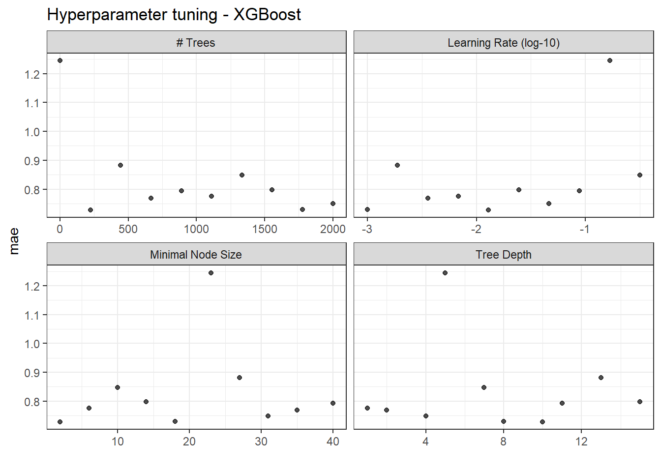

Show the code

XGB_results$final_wf_xgb # optimized hyperparameters

══ Workflow ════════════════════════════════════════════════════════════════════
Preprocessor: Recipe
Model: boost_tree()

── Preprocessor ────────────────────────────────────────────────────────────────
2 Recipe Steps

• step_mutate_at()
• step_dummy()

── Model ───────────────────────────────────────────────────────────────────────
Boosted Tree Model Specification (regression)

Main Arguments:
  trees = 223
  min_n = 2
  tree_depth = 10
  learn_rate = 0.0129154966501488

Computational engine: xgboost

Show the code

XGB_VIP <- XGB_results$xgb_vip # variable importance plot
XGB_VIP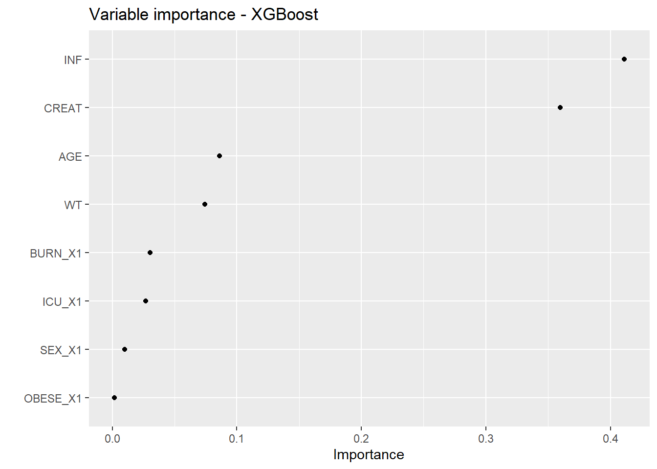

Show the code

ggsave(filename = here("Figures/S16a.jpg"),
       plot = XGB_VIP,
       width = 8, height = 6, dpi = 600)

final_xgb_fit <- XGB_results$final_xgb_fit

Show the code

test_XGB <- openMIPD::xgb_test(final_fit = final_xgb_fit, test = test_preprocessed)

Show the code

ta_results_XGB <- explore_predictions(data = test_XGB, DOSE_PRED = "XGBoost")
ta_results_XGB$target_attainment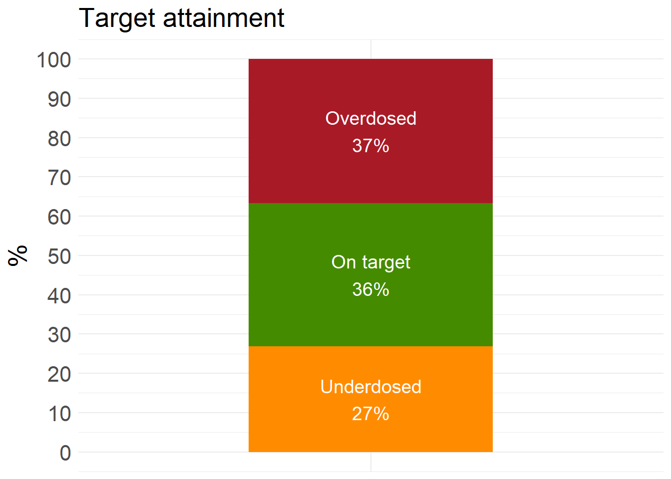

Show the code

ta_results_XGB$summary_stats

# A tibble: 2 × 10
  Prediction_correctness Count Obese mean_CREAT sd_CREAT mean_WT sd_WT mean_AGE
  <chr>                  <int> <int>      <dbl>    <dbl>   <dbl> <dbl>    <dbl>
1 Correct                  219    77      1.01     0.560    83.5  18.2     62.1
2 Incorrect                381   140      0.917    0.587    84.9  19.0     58.6
# ℹ 2 more variables: sd_AGE <dbl>, Proportion <dbl>

9.2 Random forest

A decision tree is a model that represents possible decision paths in a schematic tree-like structure. In regression trees, node splitting is done to minimize intra-group variance. In classification trees, node purity can be measured using the Gini index, where f is the frequency of observations:

\[ \text{Gini index} = 2 \cdot f \cdot (1 - f) \]

Introduced in 2001, Random Forest (RF) is a machine learning method based on an ensemble of decision trees. It uses the bootstrap aggregating algorithm (commonly known as bagging). The performance of an RF model is measured by prediction error, which corresponds to the mean squared error (MSE) for regression problems. Random Forest helps reduce variance, making it suitable for unstable, unbiased data.

Hyperparameters to define:

Number of trees (typically around 400)
mtry – the number of variables considered at each node. Default value is \(\sqrt{\text{number of predictors}}\)
Number of observations in the terminal node (leaf)

Show the code

RF_results <- openMIPD::rf_train(train = train_preprocessed, continuous_cov = c("WT", "CREAT", "AGE", "INF"), categorical_cov = c("BURN", "OBESE", "SEX", "ICU"))

A variable importance plot is generated which show the contribution of different predictors to the results. Also, the tuning and hyperparameter optimization is visualized.

Show the code

RF_results$tune_plot_rf # tuning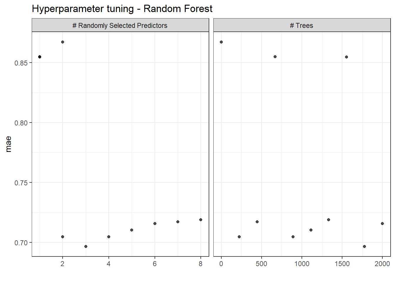

Show the code

RF_results$final_wf_rf # optimized hyperparameters

══ Workflow ════════════════════════════════════════════════════════════════════
Preprocessor: Recipe
Model: rand_forest()

── Preprocessor ────────────────────────────────────────────────────────────────
2 Recipe Steps

• step_mutate_at()
• step_dummy()

── Model ───────────────────────────────────────────────────────────────────────
Random Forest Model Specification (regression)

Main Arguments:
  mtry = 3
  trees = 1777

Engine-Specific Arguments:
  importance = impurity

Computational engine: ranger

Show the code

RF_VIP <- RF_results$rf_vip # variable importance plot
RF_VIP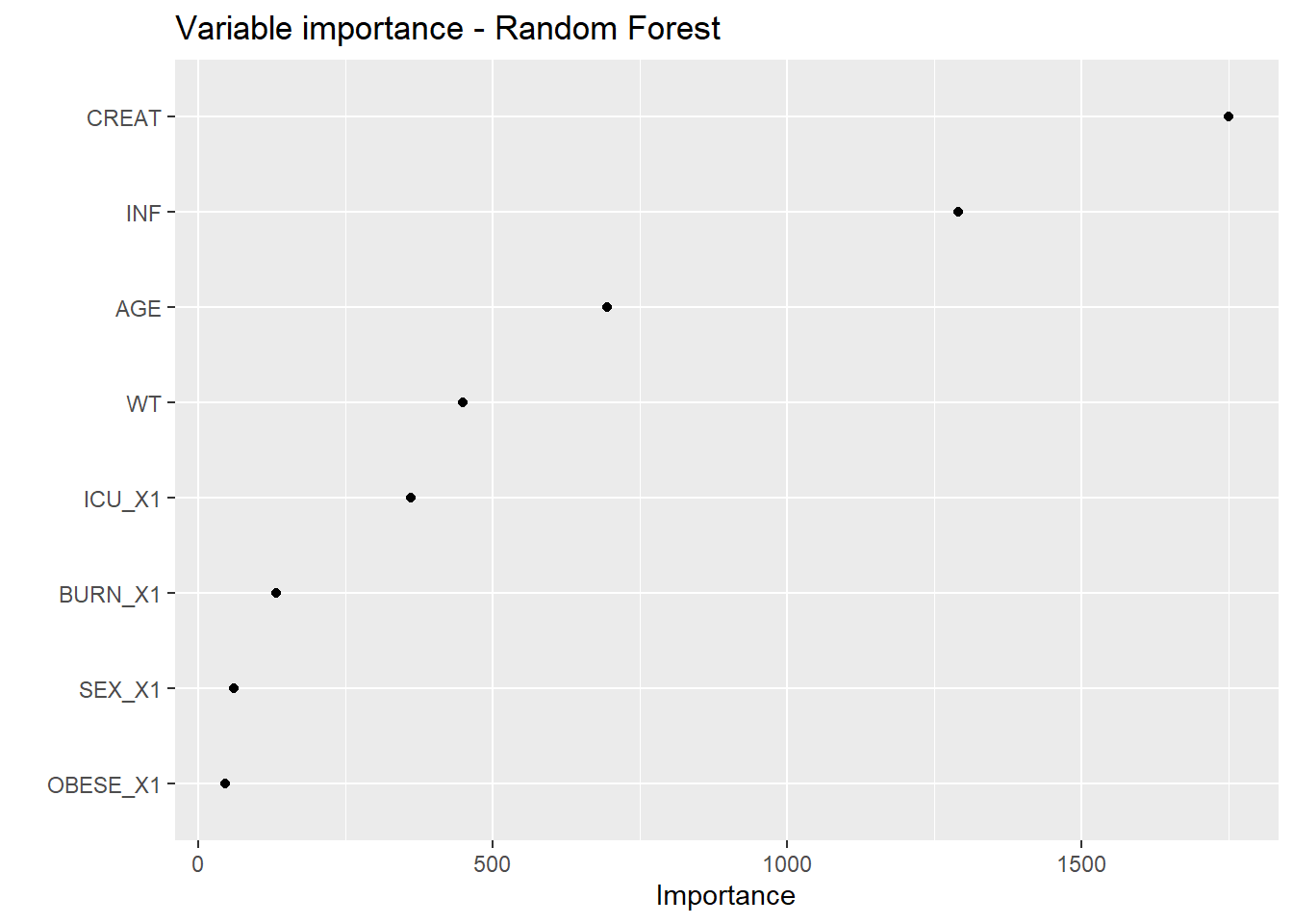

Show the code

ggsave(filename = here("Figures/S16b.jpg"),
       plot = RF_VIP,
       width = 8, height = 6, dpi = 600)
final_rf_fit <- RF_results$final_rf_fit

Show the code

test_RF <- openMIPD::rf_test(final_fit = final_rf_fit, test = test_preprocessed)

Show the code

ta_results_RF <- explore_predictions(test_RF, DOSE_PRED = "RF")
ta_results_RF$target_attainment

Show the code

ta_results_RF$summary_stats

# A tibble: 2 × 10
  Prediction_correctness Count Obese mean_CREAT sd_CREAT mean_WT sd_WT mean_AGE
  <chr>                  <int> <int>      <dbl>    <dbl>   <dbl> <dbl>    <dbl>
1 Correct                  224    69      1.03     0.589    82.0  17.9     63.2
2 Incorrect                376   148      0.905    0.569    85.8  19.0     58.0
# ℹ 2 more variables: sd_AGE <dbl>, Proportion <dbl>

9.3 Support Vector Machine

Introduced in 1995, Support Vector Machines (SVM) classify data by finding a hyperplane that maximizes the distance between classes in a multi-dimensional space. SVM regression predicts a continuous target by fitting a function with a tolerance for small deviations from the true values and penalizing large errors. SVM regression can capture non-linear relationships and is less sensible to outliers compared to linear regression. Unlike K-Nearest Neighbors (KNN), SVM is effective for high-dimensional data.

Cost – regularization parameter that determines the weight given to classification errors. If cost increases, tolerance for classification errors decreases. A smaller cost improves generalizability.
σ – controls the shape of the decision boundary. A smaller value captures local trends better but may lead to overfitting and reduced generalizability.

Show the code

SVM_results <- openMIPD::svm_train(train = train_preprocessed, continuous_cov = c("WT", "CREAT", "AGE", "INF"), categorical_cov = c("BURN", "OBESE", "SEX", "ICU"))

Show the code

SVM_results$tune_plot_svm # tuning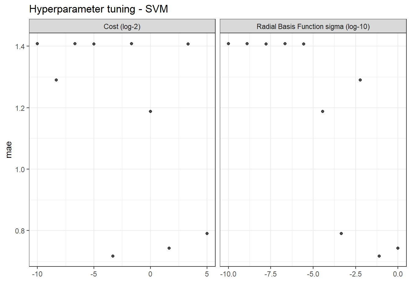

Show the code

SVM_results$final_wf_svm # optimized hyperparameters

══ Workflow ════════════════════════════════════════════════════════════════════
Preprocessor: Recipe
Model: svm_rbf()

── Preprocessor ────────────────────────────────────────────────────────────────
3 Recipe Steps

• step_mutate_at()
• step_dummy()
• step_normalize()

── Model ───────────────────────────────────────────────────────────────────────
Radial Basis Function Support Vector Machine Model Specification (regression)

Main Arguments:
  cost = 0.0992125657480125
  rbf_sigma = 0.0774263682681128

Computational engine: kernlab

Show the code

final_svm_fit <- SVM_results$final_svm_fit

Show the code

test_SVM <- openMIPD::svm_test(final_fit = final_svm_fit, test = test_preprocessed)

Show the code

ta_results_SVM <- explore_predictions(test_SVM, DOSE_PRED = "SVM")
ta_results_SVM$target_attainment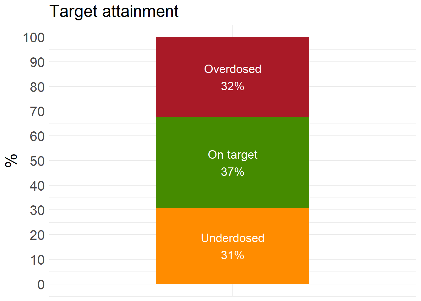

Show the code

ta_results_SVM$summary_stats

# A tibble: 2 × 10
  Prediction_correctness Count Obese mean_CREAT sd_CREAT mean_WT sd_WT mean_AGE
  <chr>                  <int> <int>      <dbl>    <dbl>   <dbl> <dbl>    <dbl>
1 Correct                  222    84      0.987    0.543    84.7  19.2     61.3
2 Incorrect                378   133      0.929    0.598    84.2  18.4     59.1
# ℹ 2 more variables: sd_AGE <dbl>, Proportion <dbl>

9.4 K-nearest neighbors (KNN)

KNN is a simple, non-parametric algorithm that is less sensitive to outliers and is used to create clusters and make predictions based on the similarity of data points. The disadvantage of KNN is that the algorithm can take a long time to run, and it is less suited for high-dimensional data.

The value of k is determined through 10-fold cross-validation.
The distance is calculated between all data points and the target point.
The k nearest neighbors are selected.
The average of the target values of these nearest neighbors will be the prediction for the given point.

The most commonly used distance metrics are as follows:

Euclidean Distance: The most commonly used; a straight line connecting two points in vector space. This distance is well-suited for outliers and noise but less suitable for data with different scales or high dimensionality. \[ d(x, y) = \sqrt{(x - y)^2} \]
Manhattan Distance: Well-suited for categorical data and high-dimensional data. It is less suitable for data with different scales.

\[ d(x, y) = |x - y| \]

Minkowski Distance: A generalization of the two previous distances. It has an additional parameter, p, that controls the importance given to differences between data points. If p = 2, it becomes the Euclidean distance, and if p = 1, it becomes the Manhattan distance. This distance is suitable for mixed data but is less interpretable, and the value of p needs to be defined.

\[ d(x, y) = \left| (x - y)^p \right|^{1/p} \]

Euclidean distance is the default distance used and it is the most interpretable and intuitive. Hyperparameters to define:

k
p (if Minkowski distance is used)

Show the code

KNN_results <- openMIPD::knn_train(train = train_preprocessed, continuous_cov = c("WT", "CREAT", "AGE", "INF"), categorical_cov = c("BURN", "OBESE", "SEX", "ICU"))

Show the code

KNN_results$tune_plot_knn # tuning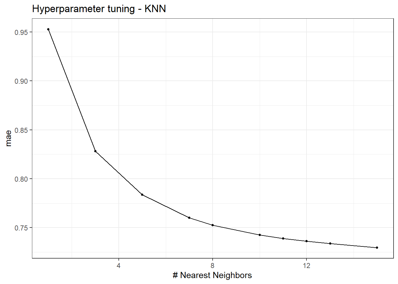

Show the code

KNN_results$final_wf_knn # optimized hyperparameters

══ Workflow ════════════════════════════════════════════════════════════════════
Preprocessor: Recipe
Model: nearest_neighbor()

── Preprocessor ────────────────────────────────────────────────────────────────
3 Recipe Steps

• step_mutate_at()
• step_dummy()
• step_normalize()

── Model ───────────────────────────────────────────────────────────────────────
K-Nearest Neighbor Model Specification (regression)

Main Arguments:
  neighbors = 15

Computational engine: kknn

Show the code

final_knn_fit <- KNN_results$final_knn_fit

Show the code

test_KNN <- openMIPD::knn_test(final_fit = final_knn_fit, test = test_preprocessed)

Show the code

ta_results_KNN <- explore_predictions(test_KNN, DOSE_PRED = "KNN")
ta_results_KNN$target_attainment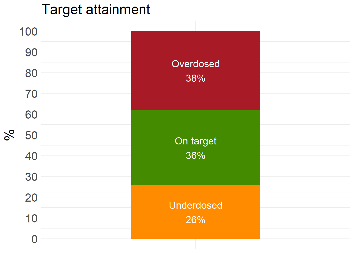

Show the code

ta_results_KNN$summary_stats

# A tibble: 2 × 10
  Prediction_correctness Count Obese mean_CREAT sd_CREAT mean_WT sd_WT mean_AGE
  <chr>                  <int> <int>      <dbl>    <dbl>   <dbl> <dbl>    <dbl>
1 Correct                  218    77      1.02     0.621    82.8  19.5     62.8
2 Incorrect                382   140      0.909    0.550    85.3  18.2     58.3
# ℹ 2 more variables: sd_AGE <dbl>, Proportion <dbl>

9.5 Stacking

The blend_predictions function determines how member model output will ultimately be combined in the final prediction by fitting a Lasso model on the data stack, predicting the true assessment set outcome using the predictions from each of the candidate members. Candidates with nonzero stacking coefficients become members.

These plots the meta-learning model over a predefined grid of lasso penalty values and uses an internal resampling method to determine the best value. The autoplot() method, shown helps us understand if the default penalization method was sufficient. It can also be used to visualize the contribution of each model type.

Show the code

amox_cmin <- stacks() %>%
    add_candidates(XGB_results$tune_res_xgb) %>%
    add_candidates(SVM_results$tune_res_svm) %>%
    add_candidates(RF_results$tune_res_rf) %>%
    add_candidates(KNN_results$tune_res_knn)
  
  conflicted::conflicts_prefer(brulee::coef)
  
  set.seed(1234)
  amox_cmin_ens <- amox_cmin %>% blend_predictions()
  
  # fit ensembled members
  set.seed(1234)
  amox_cmin_ens <- amox_cmin_ens %>% fit_members()

To evaluate training, the evolution of metrics with the number of members and the contribution of different stacking members are plotted.

Show the code

  # Stacking plots
  stacking_autoplot_default <- autoplot(amox_cmin_ens)
  stacking_members_plot <- autoplot(amox_cmin_ens, type = "members")
  stacking_weights_plot <- autoplot(amox_cmin_ens, type = "weights")
  ggsave(filename = here("Figures/S17.jpg"),
       plot = stacking_weights_plot,
       width = 8, height = 6, dpi = 600)
  
  stacking_autoplot_default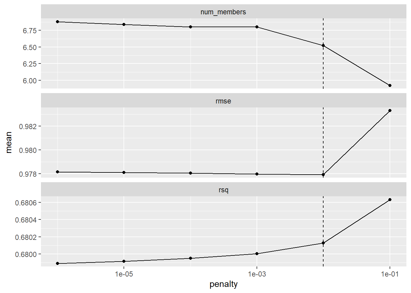

Show the code

  stacking_members_plot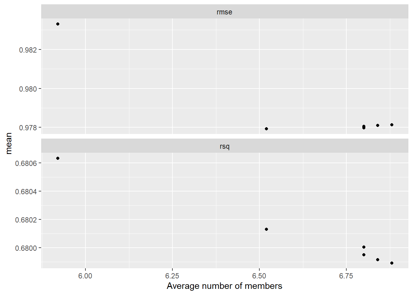

Show the code

  stacking_weights_plot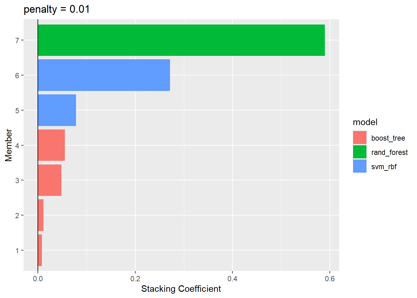

Show the code

  # Make predictions with stacking
  stack_preds <- predict(amox_cmin_ens, new_data = test_preprocessed) %>%
    dplyr::pull(.pred)

Target attainment and corresponding statistics are calculated for the predictions.

Show the code

  # Add stacking to the test table
  test_STACK <- test_preprocessed %>%
    dplyr::mutate(
      STACK = exp(stack_preds) * (II / 24)
    )
  
ta_results_STACK <- explore_predictions(test_STACK, DOSE_PRED = "STACK")
ta_results_STACK$target_attainment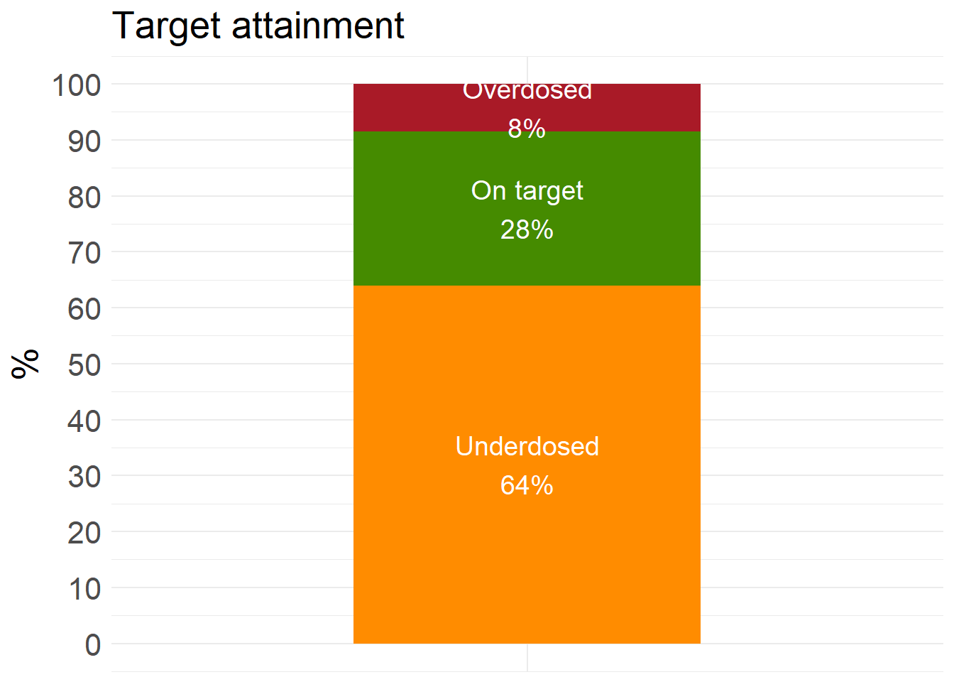

Show the code

ta_results_STACK$summary_stats

# A tibble: 2 × 10
  Prediction_correctness Count Obese mean_CREAT sd_CREAT mean_WT sd_WT mean_AGE
  <chr>                  <int> <int>      <dbl>    <dbl>   <dbl> <dbl>    <dbl>
1 Correct                  165    51      0.983    0.555    80.5  16.7     66.2
2 Incorrect                435   166      0.938    0.588    85.9  19.2     57.5
# ℹ 2 more variables: sd_AGE <dbl>, Proportion <dbl>