6  Simulation of concentrations and secondary PK parameters

library(mrgsolve)
library(here)
library(tidyverse)
library(mapbayr)
library(MESS)
library(ggplot2)
library(dplyr)
library(patchwork) # To put different plots on the same grid
library(tableone)
library(knitr)
conflicted::conflicts_prefer(dplyr::filter)
conflicted::conflicts_prefer(dplyr::select)

The objective is to simulate concentrations and secondary PK parameters (Cmax, Cmin & AUC) using 4 validated PopPK models for amoxicillin. The 4 papers are:

• Carlier et al. (2013)

• Fournier et al. (2018)

• Mellon et al. (2020)

• Rambaud et al. (2020)

The original Rambaud model was non-parametric which was approximated using a parametric model (details in “Rambaud_validation.html”).

The only route of administration is intraveinous infusion.

Three types of infusion are simulated:

• intermittent (duration = 0.5 h),

• extended (1-2 hours),

• continuous .

There are 8 different dosing schemes. For each model cohort the dosing scheme that was in the original article is used for simulation. For patients with renal failure (IR = CRCL < 30 mL/min), a different dosing scheme is applied if it is explicited in the articles (i. e. Carlier, Fournier). For Mellon, there was a single administration in the original model. To have a dosing scheme compatible with the clinical context in which we want to apply our methods, administration frequency is set to every 6 h for intermittent administrations. ID means a set of covariates, not a subject (to make data manipulation easier later).

144 observations are simulated for each subject to have a sufficient number of observations after the first dose, as well as during a steady-state interdose interval. Observations are simulated for the period between the first and second doses and for the same duration for the first interdose interval that is entirely at steady-state. The number of observations has been determined to have at least three observations during the first interdose interval for all dosing schemes. For example, in the case of an intermittent infusion of 0.5 g q6h, there is an observation in each 5 minutes between 0 and 6 h & between 24 h and 30 h (if steady-state is reached at 22 h). This means, that not only the dosing grid changes for each dosing scheme, but the observation grid as well.

here::i_am("Simulations/concentrations_simulation.qmd")
# Import or generate the file with the covariates (COV)
COV <- read.csv(here("Data/COV.csv"), quote = "")
set.seed(1991)

First, the dataset needs to be created with all the information that mrgsolve needs for the simulation. In the function create_dosing_data, the input data is created for all the lines that contain an administered dose.

# Function to create dosing grid (lines where there is an administered dose)
create_dosing_data <- function(id_range, amt, ii, rate, cmt, time_seq) {
  COV1 <- COV %>% dplyr::filter(ID %in% id_range)
  
  ID <- id_range            # ID range for the regimen
  
  # Create base dosing data
  dosing_data <- data.frame(
    ID = ID,
    amt = rep(amt, length(ID)),   # Dose amount in mg
    ii = rep(ii, length(ID)),     # Interdose interval in h
    rate = rep(rate, length(ID)), # Infusion rate
    evid = rep(1, length(ID)),    # EVID
    cmt = cmt                     # Compartment
  )
  
  # Add covariates from COV.csv
  dosing_data <- cbind(dosing_data, COV1[, setdiff(names(COV1), "ID")])
  
  # Repeat dosing data for all time points
  dosing_repeated <- dosing_data[rep(1:nrow(dosing_data), each = length(time_seq)), ]
  time <- rep(time_seq, times = length(ID))
  
  # Combine with time
  final_dosing_data <- cbind(dosing_repeated, time)
  return(final_dosing_data)
}

Then, the information is created for all the lines, that do not contain a dose, but an observation. The latest possible time is 120 h, as amoxicillin has a short half life and all subjects have had a complete steady-state dosing interval by then.

# Function to create observation grid (lines with concentration measurement)
create_observation_data <- function(id_range, obs_length) {
  COV1 <- COV %>% dplyr::filter(ID %in% id_range)
 # Extract covariates for the specified range
  ID <- id_range            # ID range for the regimen
  
  # Create base observation data (as these are lines with concentrations, AMT, II, RATE and EVID are always 0)
  obs_data <- data.frame(
    ID = ID,                     # ID meaning a set of covariates
    amt = rep(0, length(ID)),    # Dose amount in mg
    ii = rep(0, length(ID)),     # Interdose interval in h
    rate = rep(0, length(ID)),   # Infusion rate
    evid = rep(0, length(ID)),   # EVID
    cmt = "CENTRAL"              # Central compartment
  )
  
  # Add covariates
  obs_data <- cbind(obs_data, COV1[, setdiff(names(COV1), "ID")])
  
  # Repeat observation data for all observation times
  obs_repeated <- obs_data[rep(1:nrow(obs_data), each = obs_length), ]
  time <- rep(seq(from = 0, to = 120, length.out = obs_length), times = length(ID))   # Latest possible time is 120 h as amoxicillin has a short half life
  
  # Combine with time
  final_obs_data <- cbind(obs_repeated, time)
  return(final_obs_data)
}

To remove outliers, the non-physiological PK parameter values are resimulated (at most 100 times per value) using the simeta function of mrgsolve. A central volume of distribution smaller than 3 L (the volume of plasma) and a clearance higher than 180 L/h (normal blood flow) is considered non-physiological. (However, the maximum simulated clearance is around 100 L/h, so its resimulation is unnecessary.)

Simulations are done using the mrgsolve models in .cpp format. To find the interdose interval which is entirely in steady-state, first, the time to reach steady state (TSS) has to be calculated. \[ K_{10} = \frac{CL}{V_c} \]

\[ K_{12} = \frac{Q}{V_c} \]

\[ K_{21} = \frac{Q}{V_p} \]

\[ L_2 = \frac{ \left( K_{10} + K_{12} + K_{21} \right) - \sqrt{ \left( K_{10} + K_{12} + K_{21} \right)^2 - 4 K_{10} K_{21} } }{2} \] \[ t_{1/2} = \frac{ln(2)}{L_2} \] We can consider that steady state is reached when the concentration is 90 % of the steady state concentration, which corresponds to a time of 3.3 times the half life ( as \(1 - e^{(-k_e \cdot t)} = 0.9\) ).

First, concentrations are simulated for all data points between 0 and 120 h, then the results are filtered to choose the first interdose interval and the first interdose interval entirely in steady-state.

# Function to simulate based on mrgsolve models
simulate_mrgsim <- function(sim_final, model, interval) {
  sim_results <- mrgsim(model, sim_final) %>% as.data.frame()
  
  return(sim_results)
}

Then, the filtered dataset, and the covariates will be put together, and the observation and dosing grids will be simulated based on the functions defined earlier. The dosing scheme is added as three columns (DOSE, FREQuency, DURation). Each model control stream is used two times for each simulation. Once, to simulate IPRED and Y (and \(Cmax_{\text{ind}}\), \(Cmin_{\text{ind}}\) and \(AUC_{\text{ind}}\) which are based on IPRED), then a second time, the omega matrix is set to 0 to simulate PRED (and CMAX_PRED and AUC_PRED based on PRED). PRED are typical concentrations which do not contain inter-individual variability. IPRED has inter-individual variability incorporated, and Y has both inter-and intra-individual variability.

# Function to merge covariates and finalize
finalize_results <- function(sim_results, id_range, model, dose, freq, dur) {
  COV1 <- COV %>% dplyr::filter(ID %in% id_range)
  
  # Merge with simulation results
  result <- merge(sim_results, COV1, by = "ID", all.x = TRUE)
  
  result <- result %>%
    mutate(MODEL = model, DOSE_ADM = dose, FREQ = freq, DUR = dur) %>%
    distinct(ID, TIME = time, .keep_all = TRUE)
  
  return(result)
}

generate_model_regimen <- function(model_name, cpp_file, regimens, sim_dur,cohort_name) {
  model <- mread(model = cpp_file)
  model_zero <- zero_re(model)
  COV <- read.csv(here("Data/COV.csv"), quote = "")

  regimen_assignments <- list()

    cohort_cov <- COV %>% filter(MODEL_COHORT == cohort_name)
    cohort_regimens <- regimens[sapply(regimens, function(x) x$model_cohort == cohort_name)]

    for (ir_value in unique(cohort_cov$IR)) {
      eligible_ids <- cohort_cov %>% filter(IR == ir_value) %>% pull(ID)

      matched_regimens <- cohort_regimens[seq_along(cohort_regimens) %% length(unique(cohort_cov$IR)) == ir_value]

      # Distribute eligible subjects evenly across relevant dosing regimens
      id_splits <- split(eligible_ids, rep(1:length(matched_regimens), length.out = length(eligible_ids)))

      for (i in seq_along(matched_regimens)) {
        matched_regimens[[i]]$assigned_ids <- id_splits[[i]]
        regimen_assignments <- append(regimen_assignments, list(matched_regimens[[i]]))
      }
    }

  # Simulate for the assigned regimens
  regimen_results <- list()
  for (regimen in regimen_assignments) {
    if (length(regimen$assigned_ids) == 0) next

    dose <- regimen$dose
    interval <- regimen$interval
    duration <- regimen$duration
    id_range <- regimen$assigned_ids

    dosing_times <- seq(0, sim_dur - interval, by = interval)
    obs_length <- (sim_dur / interval) * sim_dur + 1

    dose_data <- create_dosing_data(
      id_range = id_range,
      amt = dose,
      ii = interval,
      rate = dose / duration,
      cmt = "CENTRAL",
      time_seq = dosing_times
    )

    obs_data <- create_observation_data(id_range = id_range, obs_length = obs_length)
    sim_data <- rbind(dose_data, obs_data) %>% arrange(ID, time, desc(evid))

processed_data <- simulate_mrgsim(sim_data, model, interval)

finalized_data <- finalize_results(
      sim_results = processed_data,
      id_range = id_range,
      model = model_name,
      dose = dose,
      freq = interval,
      dur = duration
    )

    merged_data <- finalized_data
    
    regimen_results <- append(regimen_results, list(merged_data))
  }

  combined_results <- do.call(rbind, regimen_results)
  return(combined_results)
}

8 different dosing schemes are used depending on the model cohort.

# Define regimen parameters for all models. For each regimen, we take a different batch of 100 sets of covariates (defined by starting ID)
regimens <- list(
  list(model_cohort = "CARLIER", ir_group = 0, dose = 1000, interval = 6, duration = 0.5),
  list(model_cohort = "CARLIER", ir_group = 1, dose = 1000, interval = 8, duration = 0.5),
  list(model_cohort = "FOURNIER", ir_group = 0, dose = 1000, interval = 6, duration = 2),
  list(model_cohort = "FOURNIER", ir_group = 0, dose = 1500, interval = 6, duration = 1),
  list(model_cohort = "FOURNIER", ir_group = 0, dose = 2000, interval = 6, duration = 2),
  list(model_cohort = "FOURNIER", ir_group = 0, dose = 2000, interval = 8, duration = 1),
  list(model_cohort = "FOURNIER", ir_group = 1, dose = 500, interval = 8, duration = 2),
  list(model_cohort = "MELLON", ir_group = 0, dose = 1000, interval = 6, duration = 0.5),
  list(model_cohort = "RAMBAUD", ir_group = 0, dose = 12000, interval = 24, duration = 24),
  list(model_cohort = "RAMBAUD", ir_group = 0, dose = 14000, interval = 24, duration = 24)
)

# Total simulation time
sim_dur <- 120

Finally, the simulations are done with each respective model, the results are merged and a MODEL column is added to identify the model used for the simulation of each concentration.

results_Carlier <- generate_model_regimen("amox_Carlier", here("Simulations/amox_Carlier"), regimens, sim_dur,cohort_name = "CARLIER")
results_Fournier <- generate_model_regimen("amox_Fournier", here("Simulations/amox_Fournier"), regimens, sim_dur,cohort_name = "FOURNIER")
results_Mellon <- generate_model_regimen("amox_Mellon", here("Simulations/amox_Mellon"), regimens, sim_dur,cohort_name = "MELLON")
results_Rambaud <- generate_model_regimen("amox_Rambaud", here("Simulations/amox_Rambaud"), regimens, sim_dur, cohort_name = "RAMBAUD")

# Combine results from the simulation
all_results_raw <- dplyr::bind_rows(
  results_Carlier,
  results_Fournier,
  results_Mellon,
  results_Rambaud
)

# Add MODEL column indicating the model which is used for the simulation
all_results_raw <- all_results_raw %>%
  dplyr::mutate(MODEL = case_when(
    MODEL == "amox_Carlier" ~ "CARLIER",
    MODEL == "amox_Fournier" ~ "FOURNIER",
     MODEL == "amox_Mellon" ~ "MELLON",
    MODEL == "amox_Rambaud" ~ "RAMBAUD")
  ) %>%
  distinct()

# Filter based on steady-state based on the reference (true) clearance and volume
ref_values <- all_results_raw %>%
  filter(MODEL == MODEL_COHORT) %>%
  group_by(ID) %>%
  slice(1) %>%
  select(ID, Vc, CL, Q, Vp)

all_results <- all_results_raw %>%
  left_join(ref_values, by = "ID", suffix = c("", "_ref")) %>%
  mutate(K10 = CL_ref/Vc_ref,
  K12 = Q_ref/Vc_ref,
  K21 = Q_ref/Vp_ref,
  L2 = ((K10+K12+K21)-((K10+K12+K21)**2-4*K10*K21)**0.5)/2,
  TSS = ceiling((3.3 * (0.693 / L2)) / FREQ) * FREQ) %>%
  dplyr::filter((TIME >= 0 & TIME <= (0 + FREQ)) | (TIME >= TSS & TIME <= (TSS + FREQ)))

6.1 Concentrations (PRED, IPRED, Y)

Below quantification limit observations are removed (M1 method). LLOQ concentrations for each model can be found in “mrgsolve/LLOQ.txt”.

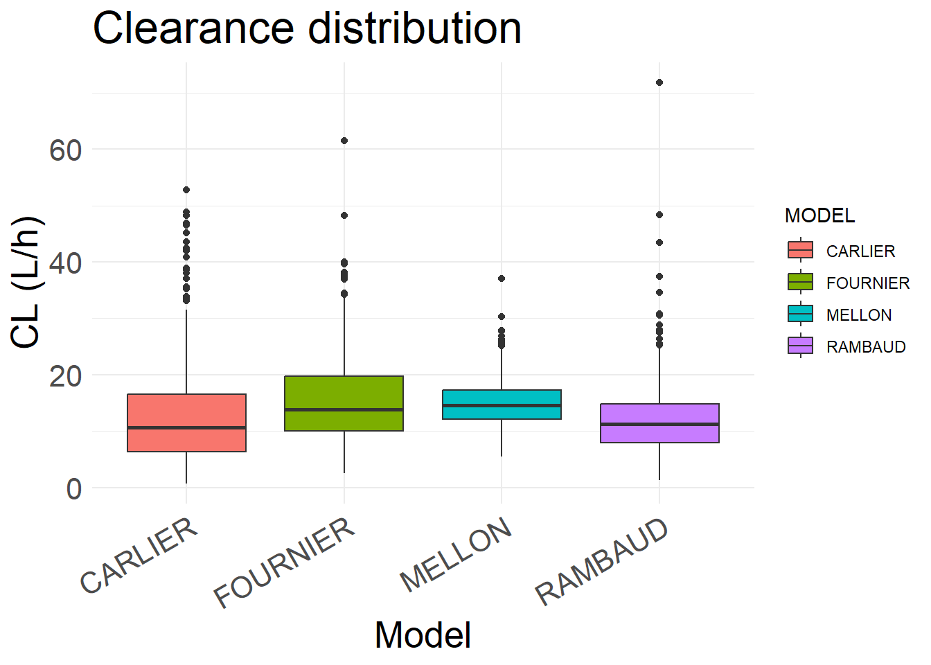
AMOX_SIM <- all_results %>%
  select(ID, TIME, IPRED, Y, WT, CREAT, BURN, ICU, OBESE, AGE, SEX, HT, BSA, MODEL, MODEL_COHORT, DOSE_ADM, FREQ, DUR, Vc, CL, TSS) %>%
  distinct()

# Dataset to plot CL
summarized_SIM <- AMOX_SIM %>%
  distinct(ID, MODEL, CL, Vc)

# Box plot for CL
plot_CL <- ggplot(summarized_SIM, aes(x = MODEL, y = CL, fill = MODEL)) +
  geom_boxplot() +
  theme_minimal() +
  labs(title = "Clearance distribution", x = "Model", y = "CL (L/h)") +
  theme(
    axis.text.x = element_text(angle = 30, hjust = 1),
    axis.text = element_text(size = 16),    
    axis.title = element_text(size = 20), 
    plot.title = element_text(size=24),
  )

plot_CL

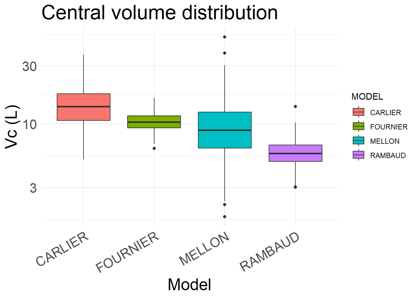
# Box plot for Vc
plot_V <- ggplot(summarized_SIM, aes(x = MODEL, y = Vc, fill = MODEL)) +
  geom_boxplot() +
  theme_minimal() +
  scale_y_log10() + 
  labs(title = "Central volume distribution", x = "Model", y = "Vc (L)") +
  theme(
    axis.text.x = element_text(angle = 30, hjust = 1),
    axis.text = element_text(size = 16),    
    axis.title = element_text(size = 20), 
    plot.title = element_text(size=24),
  )

plot_V

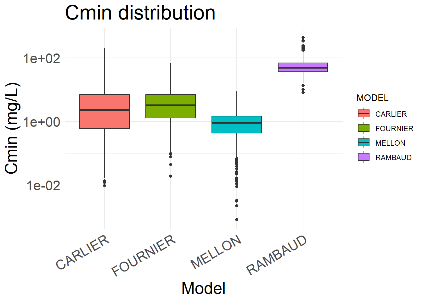
6.2 Trough concentration (Cmin)

The trough concentration is the last concentration for the steady-state interdose interval

# Add CMIN column by taking the last steady-state concentration
AMOX_CMIN1 <- AMOX_SIM %>%
  group_by(ID, MODEL) %>%
  arrange(TIME) %>%
  mutate(CMIN_IND = last(IPRED[TIME == max(TIME)])) %>%
  slice_max(TIME, n = 1, with_ties = FALSE) %>%
  ungroup() %>%
  distinct(ID, MODEL, CMIN_IND, .keep_all = TRUE) %>%
  mutate(CON = ifelse(DUR == 24, 1, 0))

  
# Box plot for CL before removing the outliers
plot_CMIN <- ggplot(AMOX_CMIN1, aes(x = MODEL, y = CMIN_IND, fill = MODEL)) +
  geom_boxplot() +
  scale_y_log10() +
  theme_minimal() +
  labs(title = "Cmin distribution", x = "Model", y = "Cmin (mg/L)") +
  theme(
    axis.text.x = element_text(angle = 30, hjust = 1),
    axis.text = element_text(size = 16),    
    axis.title = element_text(size = 20), 
    plot.title = element_text(size=24),
  )

plot_CMIN

# Create test data by taking 2400 subjects (24 from each dosing scheme and 6-6 for each model covariate cohorte per dosing scheme)
CMIN_test <- AMOX_CMIN1 %>%
  dplyr::filter(
    ID %% 100 >= 1 & ID %% 100 <= 6 |
      ID %% 100 >= 26 & ID %% 100 <= 31 |
      ID %% 100 >= 51 & ID %% 100 <= 56 |
      ID %% 100 >= 76 & ID %% 100 <= 81
  )

# Create training data by taking 7600 subjects (76 from each dosing scheme and 19-19 for each model covariate cohorte per dosing scheme)
CMIN_train <- AMOX_CMIN1 %>%
  dplyr::filter(
    ID %% 100 >= 7 & ID %% 100 <= 25 |
      ID %% 100 >= 32 & ID %% 100 <= 50 |
      ID %% 100 >= 57 & ID %% 100 <= 75 |
      ID %% 100 >= 82 & ID %% 100 <= 100
  )

# Dataset identifyer
CMIN_train_compare <- CMIN_train %>% mutate(Dataset = "Train")
CMIN_test_compare <- CMIN_test %>% mutate(Dataset = "Test")

# Combine the three datasets
combined_CMIN <- bind_rows(CMIN_train_compare, CMIN_test_compare)

# Compare the train and test sets
vars <- c("CREAT", "WT", "CMIN_IND", "CL", "Vc")
tableOne5 <- CreateTableOne(vars = vars, strata = "Dataset", data = combined_CMIN)
tableOne6 <- print(tableOne5, nonnormal = c("CREAT", "WT", "CMIN_IND", "CL", "Vc"), printToggle=F, minMax=T)

kableone(tableOne6)

	Test	Train	p	test
n	600	1875
CREAT (median [range])	0.76 [0.24, 5.32]	0.77 [0.13, 8.23]	0.410	nonnorm
WT (median [range])	80.03 [41.33, 139.60]	79.99 [47.36, 141.17]	0.884	nonnorm
CMIN_IND (median [range])	3.03 [0.00, 201.92]	2.96 [0.00, 443.50]	0.539	nonnorm
CL (median [range])	13.08 [0.68, 61.52]	12.70 [1.08, 71.87]	0.467	nonnorm
Vc (median [range])	9.60 [2.17, 38.10]	9.42 [1.73, 51.90]	0.312	nonnorm

# Export to csv
write.csv(CMIN_train, here("Data/AMOX_CMIN_OBS_TRAIN.csv"), row.names = FALSE, quote = FALSE)
write.csv(CMIN_test, here("Data/AMOX_CMIN_OBS_TEST.csv"), row.names = FALSE, quote = FALSE)

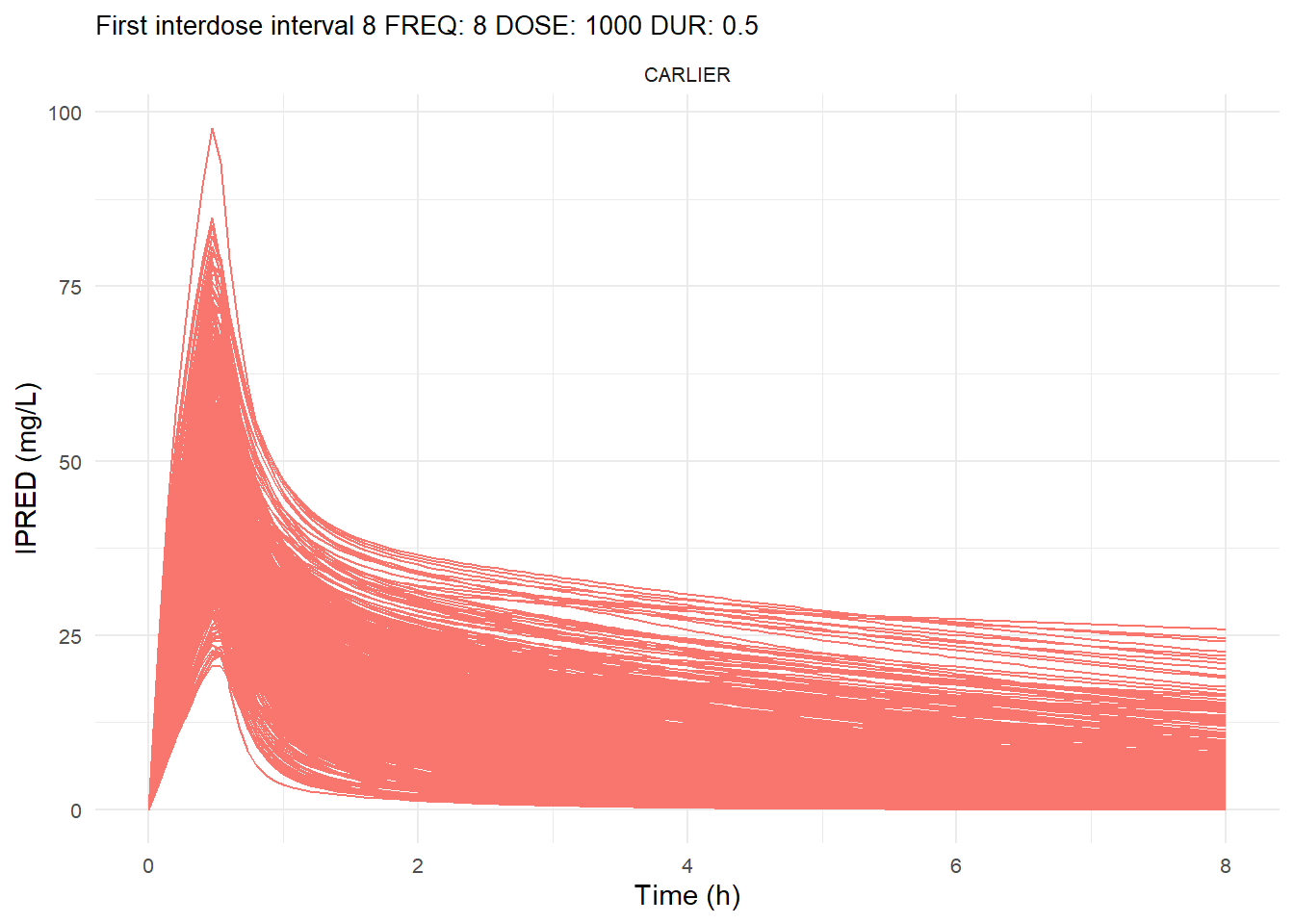
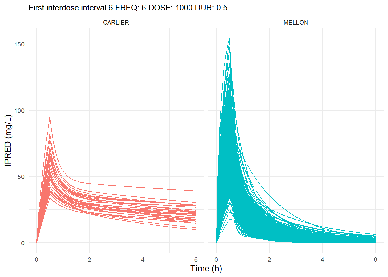
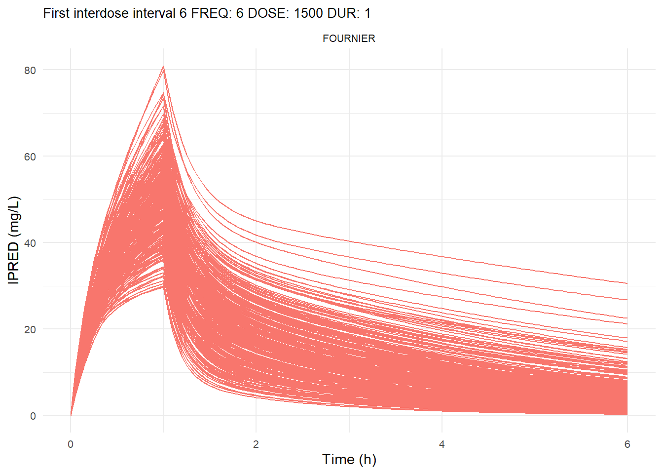
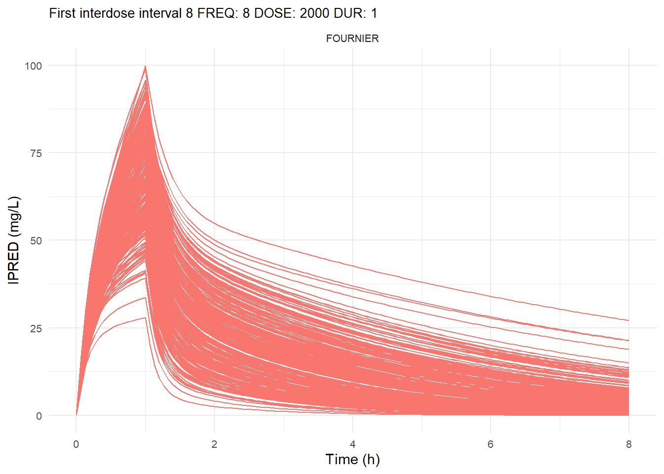
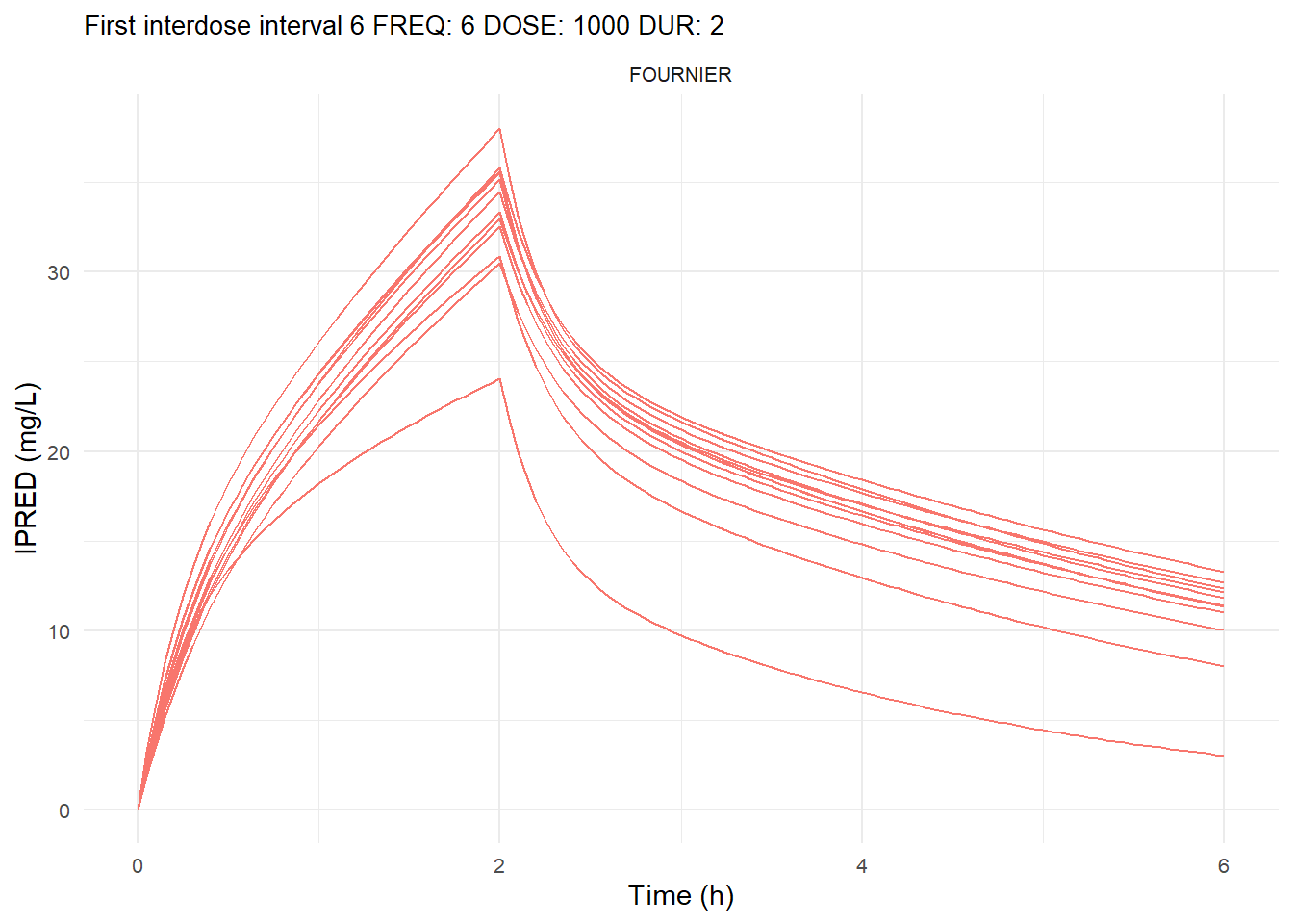
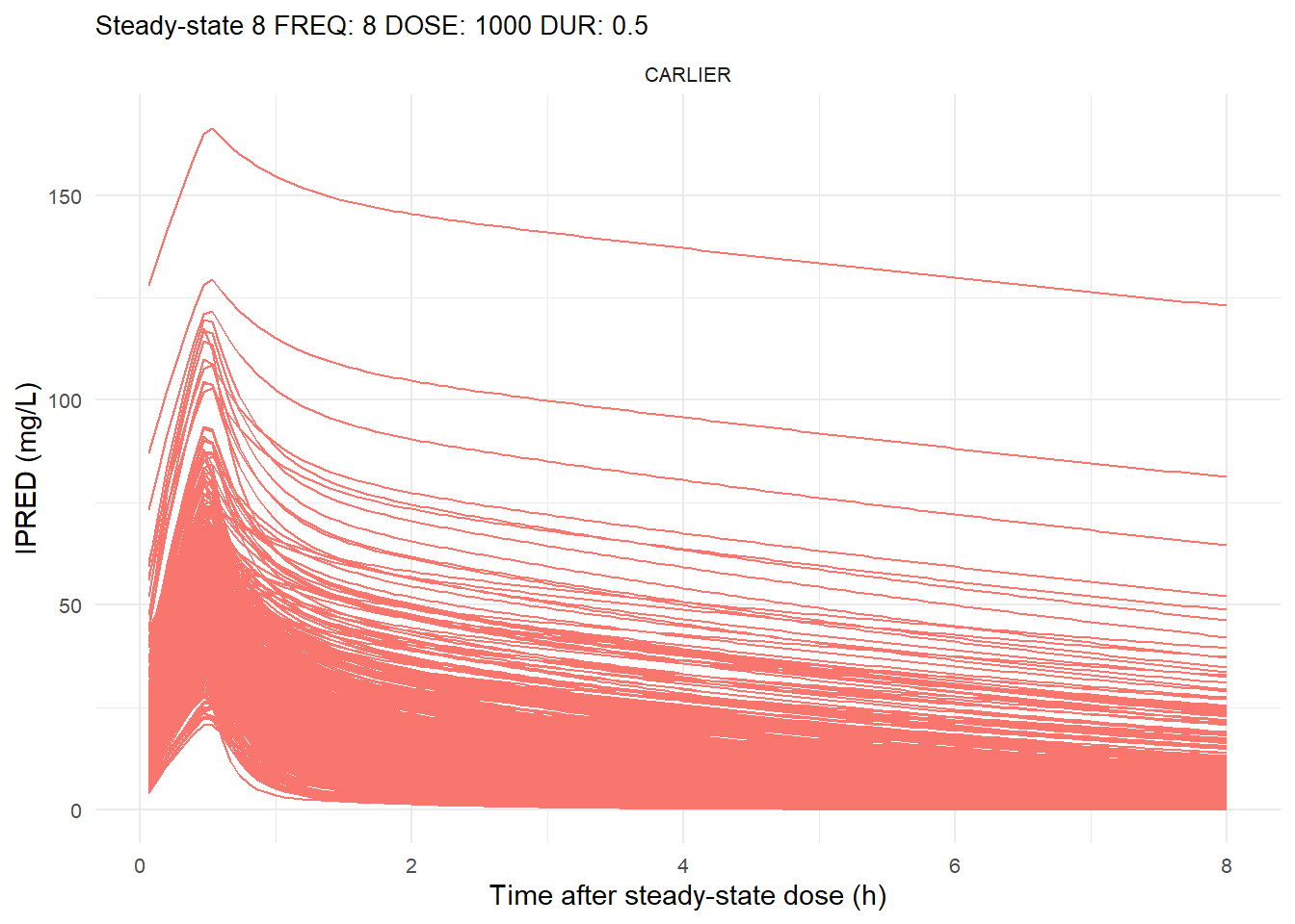
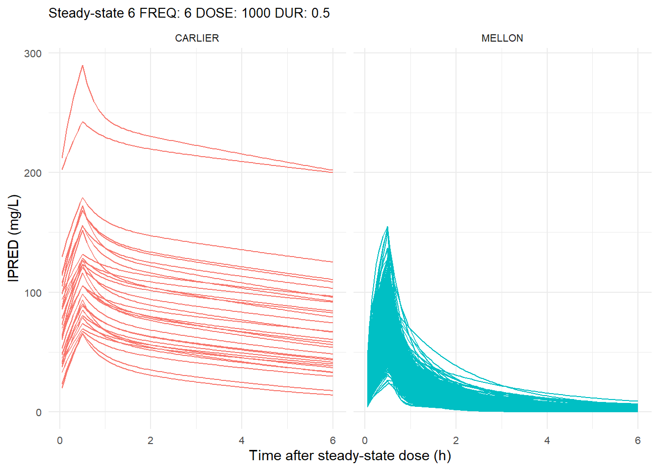
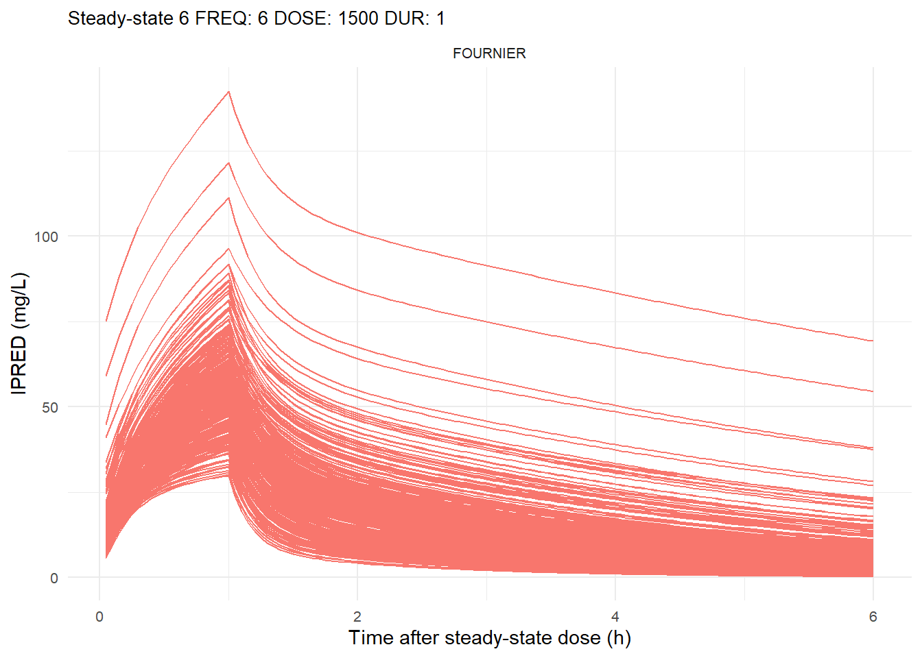
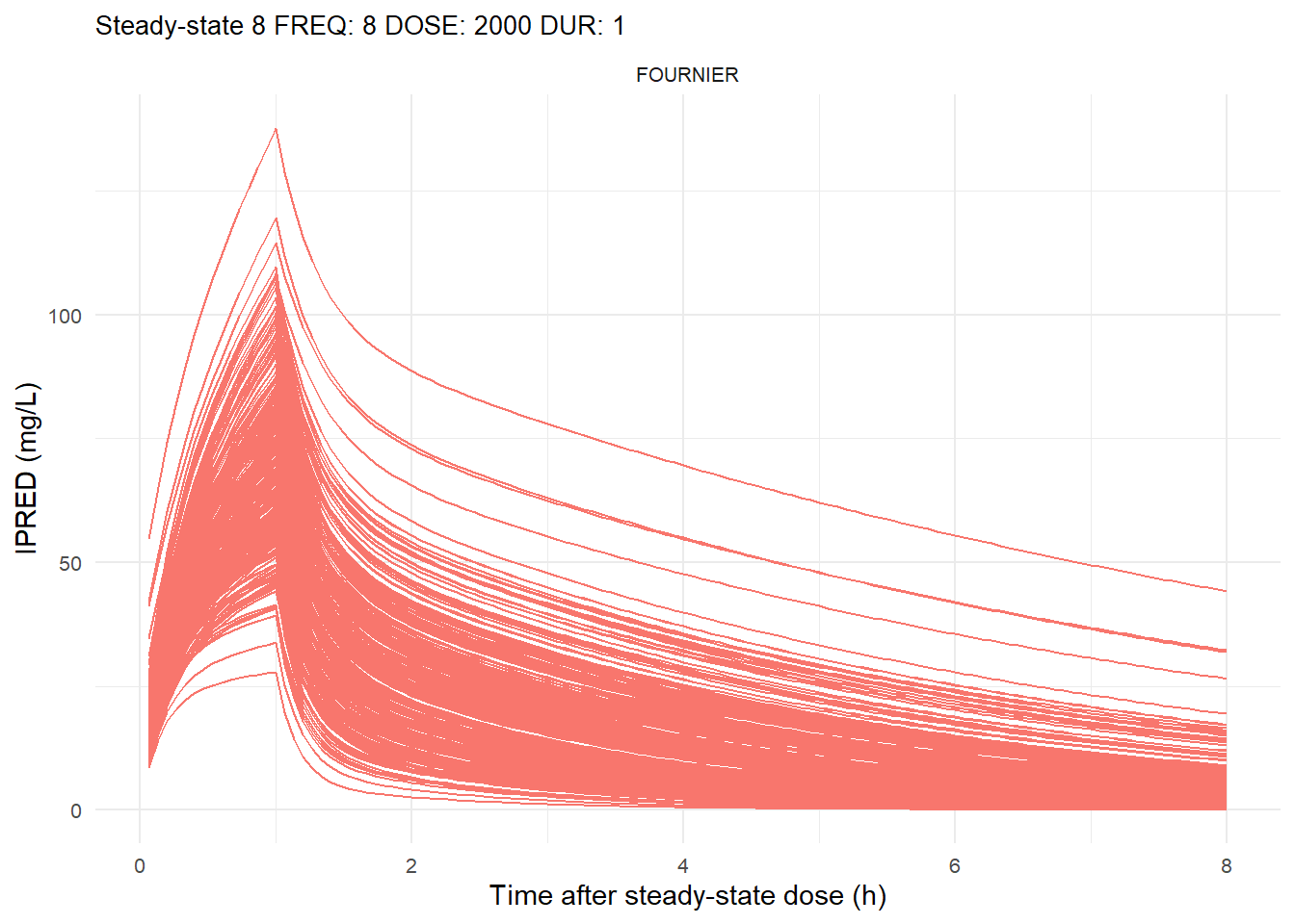
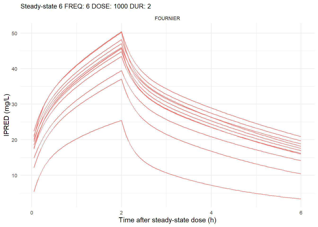
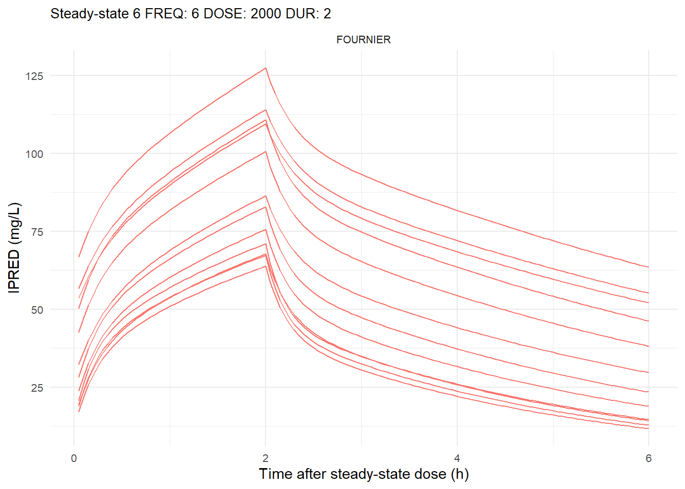
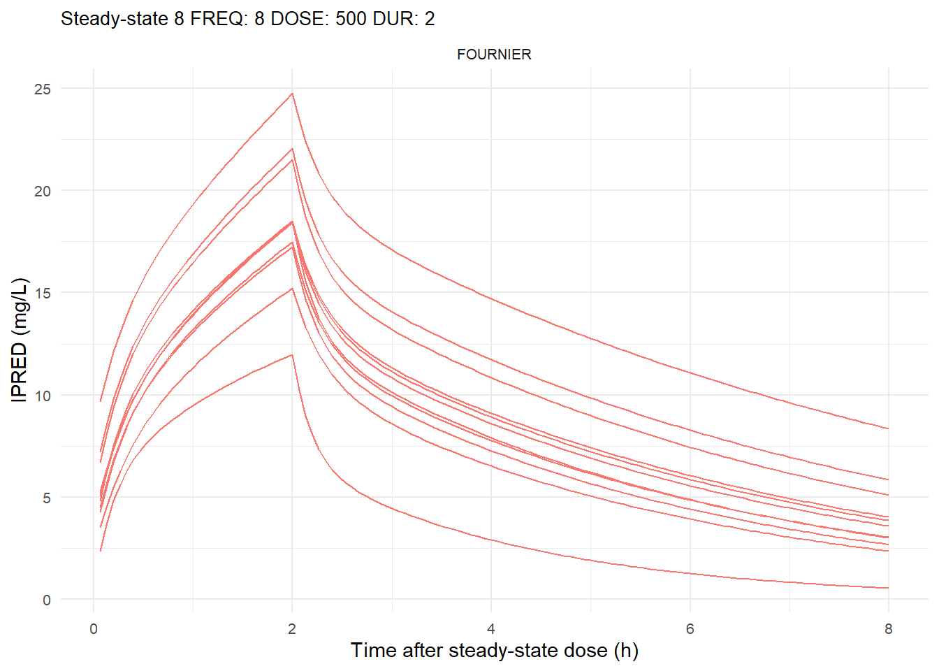
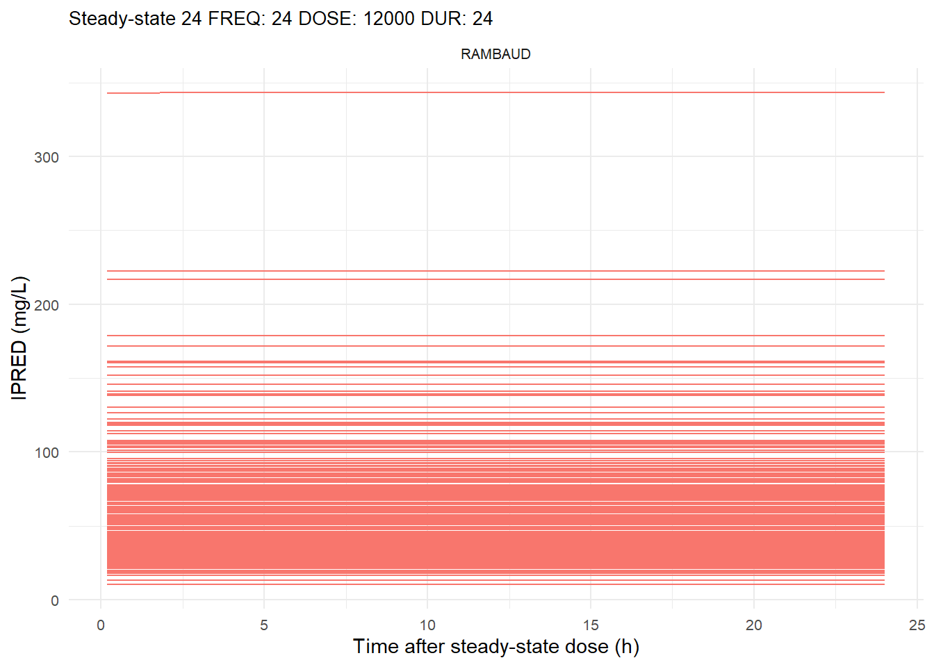
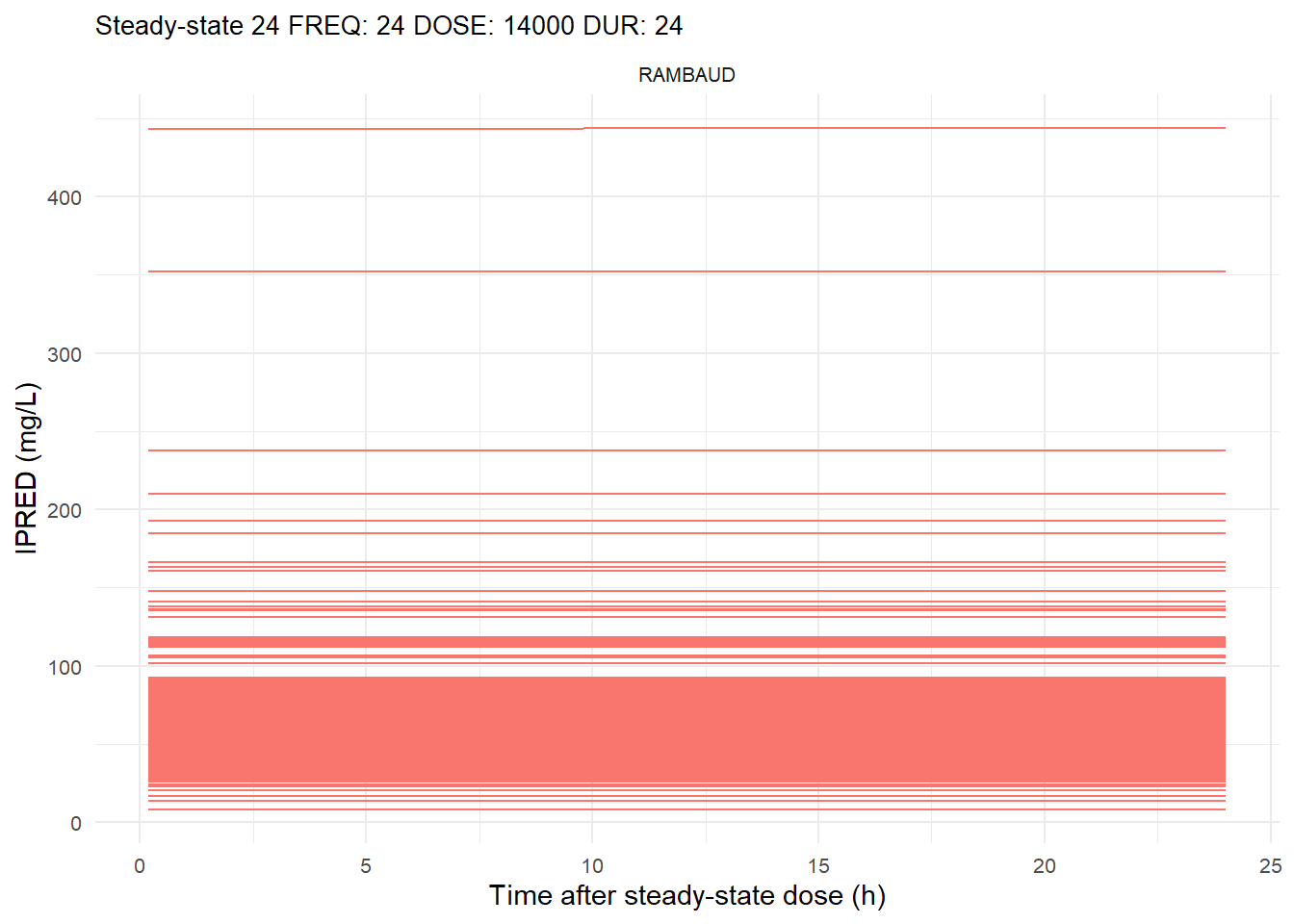
6.3 Data visualization stratified by dosing schemes

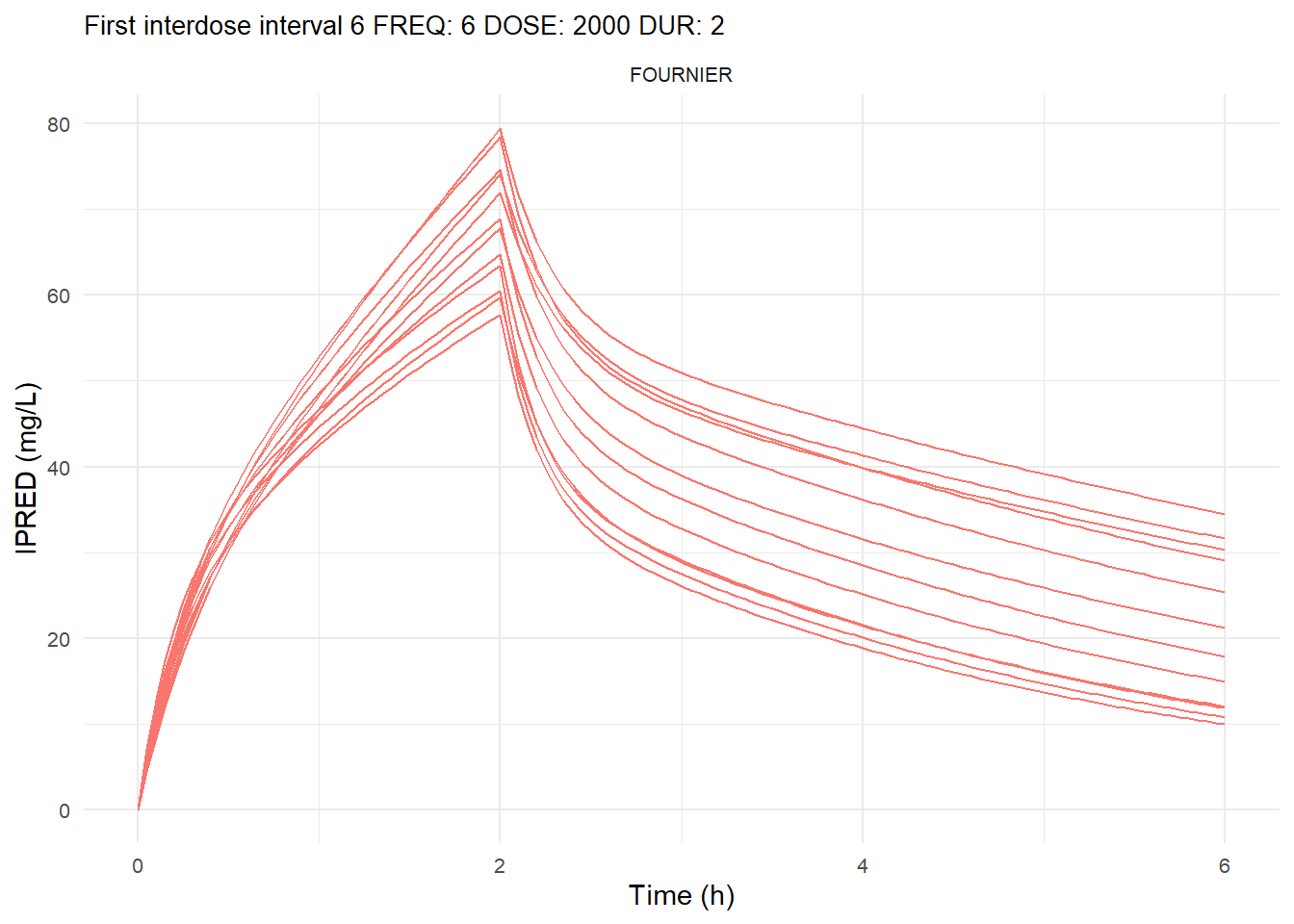
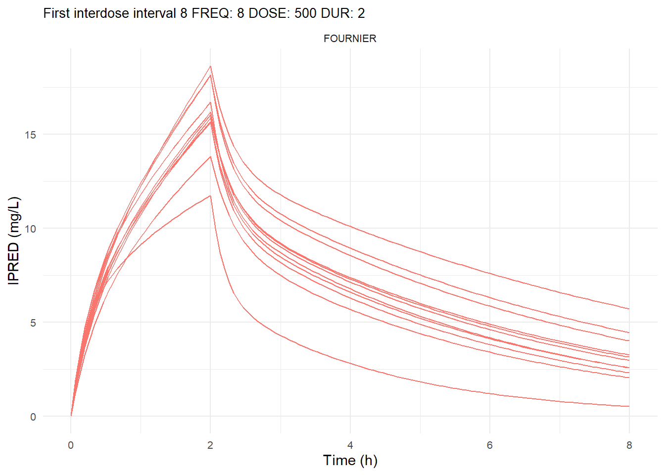
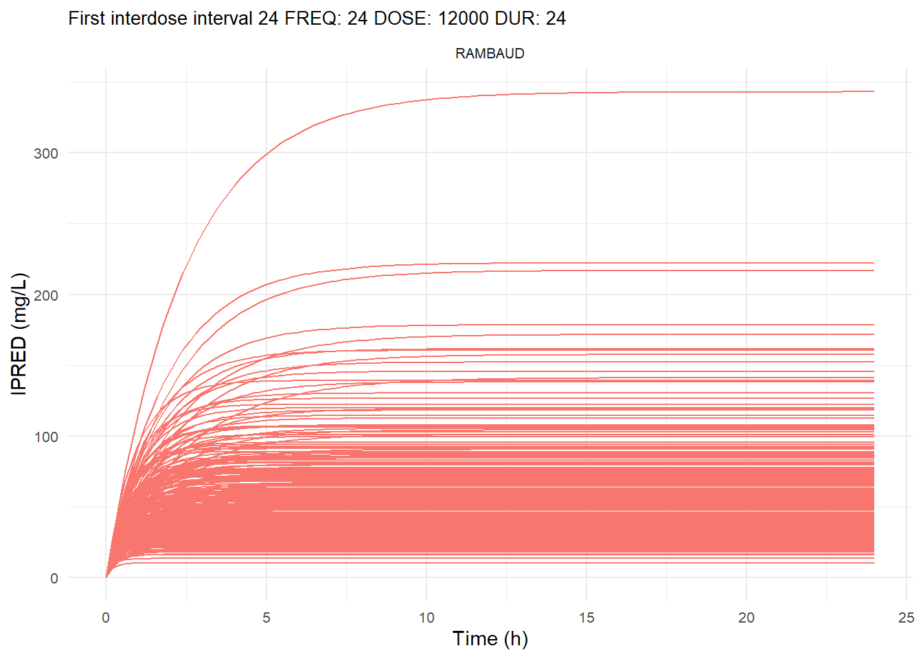
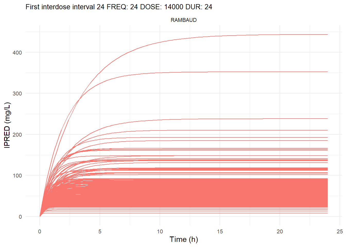
The following graphs show the individual observed concentration-time curves for the data stratified by model. One graph shows the concentration-time curves for the first interdose interval and the other graph for the interdose interval after the dose which permits to reach steady state.

# Add dosing scheme as a categorical variable (to separate dosing schemes)
data_ref <- AMOX_SIM %>%
  mutate(DOSING_SCHEME = paste("FREQ:", FREQ, "DOSE:", DOSE_ADM, "DUR:", DUR, sep = " "))

dosing_schemes <- unique(data_ref$DOSING_SCHEME)

# Loop through each dosing scheme
plot_dosing_schemes <- function(data_ref, dosing_schemes) {
  plot_list_before <- list()
  plot_list_after <- list()
  
  for (i in seq_along(dosing_schemes)) {
    scheme <- dosing_schemes[i]
    
    # Extract FREQ (=interdose interval)
    scheme_data <- subset(data_ref, DOSING_SCHEME == scheme)
    freq_value <- unique(scheme_data$FREQ)
    
    
    # Split data before and after SS
    data_before <- subset(scheme_data, TIME <= freq_value)
    data_after <- subset(scheme_data, TIME > TSS) %>%
      mutate(TIME = TIME - TSS)  # Adjust time so that it means time after SS dose
    
    # Plot for before SS
    plot_list_before[[i]] <- ggplot(data_before, aes(x = TIME, y = IPRED, color = MODEL, group = ID)) +
      geom_line() + 
      facet_wrap(~MODEL) +
      theme_minimal() + 
      labs(
        title = paste("First interdose interval", freq_value, scheme),
        x = "Time (h)",
        y = "IPRED (mg/L)",
        color = "MODEL"
      ) +
      theme(
        plot.title = element_text(size=10),
        strip.text = element_text(size = 8), 
        axis.text = element_text(size = 8),
        legend.position = "none"
      )
    
    # Plot for after SS is reached
    plot_list_after[[i]] <- ggplot(data_after, aes(x = TIME, y = IPRED, color = MODEL, group = ID)) +
      geom_line() + 
      facet_wrap(~MODEL) +
      theme_minimal() + 
      labs(
        title = paste("Steady-state", freq_value, scheme),
        x = "Time after steady-state dose (h)",
        y = "IPRED (mg/L)",
        color = "MODEL"
      ) +
      theme(
        plot.title = element_text(size=10),
        strip.text = element_text(size = 8), 
        axis.text = element_text(size = 8),
        legend.position = "none"
      )
  }
  
  list(before = plot_list_before, after = plot_list_after)
}

conc_profile_plots <- plot_dosing_schemes(data_ref, dosing_schemes)
conc_profile_plots

$before
$before[[1]]

$before[[2]]

$before[[3]]

$before[[4]]

$before[[5]]

$before[[6]]

$before[[7]]

$before[[8]]

$before[[9]]

$after
$after[[1]]

$after[[2]]

$after[[3]]

$after[[4]]

$after[[5]]

$after[[6]]

$after[[7]]

$after[[8]]

$after[[9]]

Visualization of 5th, 50th and 95th percentiles (5th and 95th percentiles in dashed)

# The data is binned to 40 bins to make it smoother
data_percentiles_ref <- data_ref %>% filter(TIME > TSS) %>%
      mutate(TIME = TIME - TSS) |> 
  mutate(TIME_bin = ntile(TIME, 40)) %>%
  group_by(DOSING_SCHEME, MODEL, TIME_bin) %>%
  summarise(
    P5 = quantile(IPRED, 0.05, na.rm = TRUE),
    P50 = quantile(IPRED, 0.50, na.rm = TRUE),
    P95 = quantile(IPRED, 0.95, na.rm = TRUE),
    TIME = median(TIME, na.rm = TRUE),
    .groups = 'drop'
  )

# Loop through each dosing scheme
plot_percentiles <- function(data_percentiles_ref, dosing_schemes) {
  library(ggplot2)
  library(patchwork)
  
  plot_list_ref <- list()
  
  for (i in seq_along(dosing_schemes)) {
    plot_list_ref[[i]] <- ggplot(
      subset(data_percentiles_ref, DOSING_SCHEME == dosing_schemes[i]),
      aes(x = TIME)
    ) +
      geom_line(aes(y = P5, color = MODEL), linetype = "dashed") +
      geom_line(aes(y = P50, color = MODEL), size = 1) +
      geom_line(aes(y = P95, color = MODEL), linetype = "dashed") +
      theme_minimal() +
      labs(
        title = paste(dosing_schemes[i]),
        x = "Time post steady-state (binned)",
        y = "IPRED (mg/L)",
        color = "MODEL"
      ) +
      theme(
        plot.title = element_text(size = 10),
        axis.text = element_text(size = 8),
        strip.text = element_text(size = 8),
        legend.position = "bottom"
      )
  }
  
  return(plot_list_ref)
}


percentile_plots <- plot_percentiles(data_percentiles_ref, dosing_schemes)

6.4 Appendix : What if you were interested in something else than Cmin ?

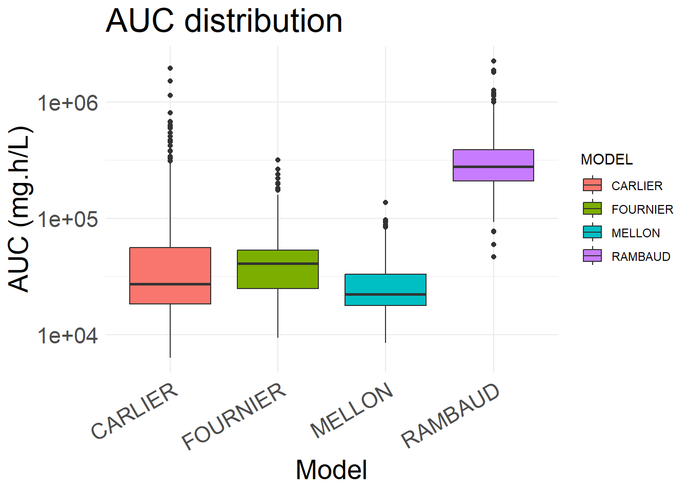
6.4.1 Exposure (AUC)

AUC is calculated based on the sum of the integrals of IPRED values and cumulated for both the steady-state and non stead-state inter-dose interval.

AMOX_AUC1 <- all_results %>%
  group_by(ID, MODEL) %>% 
  summarize(
    ID = first(ID),
    MODEL = first(MODEL),
    MODEL_COHORT = first(MODEL_COHORT),
    AUC_IND = sum(AUC, na.rm = TRUE), #total AUC (based on IPRED)
    WT = first(WT),    
    CREAT = first(CREAT), 
    BURN = first(BURN),
    ICU = first(ICU),
    OBESE = first(OBESE),
    AGE = first(AGE),
    SEX = first(SEX),
    HT = first(HT),
    DUR = first(DUR),
    FREQ = first(FREQ),
    DOSE_ADM = first(DOSE_ADM),
    TSS = first(TSS),
    Vc = first(Vc),
    CL = first(CL)
  )

summarized_AUC <- AMOX_AUC1 %>%
  distinct(ID, MODEL, AUC_IND) 

# Box plot for AUC
plot_AUC <- ggplot(summarized_AUC, aes(x = MODEL, y = AUC_IND, fill = MODEL)) +
  geom_boxplot() +
  scale_y_log10() +
  theme_minimal() +
  labs(title = "AUC distribution", x = "Model", y = "AUC (mg.h/L)") +
  theme(
    axis.text.x = element_text(angle = 30, hjust = 1),
    axis.text = element_text(size = 16),    
    axis.title = element_text(size = 20), 
    plot.title = element_text(size=24),
  )

plot_AUC

# Create test data by taking 2400 subjects (24 from each dosing scheme and 6-6 for each model covariate cohorte per dosing scheme)
AUC_test <- AMOX_AUC1 %>%
  dplyr::filter(
    ID %% 100 >= 1 & ID %% 100 <= 6 |
      ID %% 100 >= 26 & ID %% 100 <= 31 |
      ID %% 100 >= 51 & ID %% 100 <= 56 |
      ID %% 100 >= 76 & ID %% 100 <= 81
  )

# Create training data by taking 7600 subjects (76 from each dosing scheme and 19-19 for each model covariate cohorte per dosing scheme)
AUC_train <- AMOX_AUC1 %>%
  dplyr::filter(
    ID %% 100 >= 7 & ID %% 100 <= 25 |
      ID %% 100 >= 32 & ID %% 100 <= 50 |
      ID %% 100 >= 57 & ID %% 100 <= 75 |
      ID %% 100 >= 82 & ID %% 100 <= 100
  )

# Dataset identifyer
AUC_train_compare <- AUC_train %>% mutate(Dataset = "Train")
AUC_test_compare <- AUC_test %>% mutate(Dataset = "Test")

# Combine the three datasets
combined_AUC <- bind_rows(AUC_train_compare, AUC_test_compare)

# Compare the train and test sets
vars <- c("CREAT", "WT", "AUC_IND", "CL", "Vc")
tableOne <- CreateTableOne(vars = vars, strata = "Dataset", data = combined_AUC)
tableOne2 <- print(tableOne, nonnormal = c("CREAT", "WT", "AUC_IND", "CL", "Vc"), printToggle=F, minMax=T)

kableone(tableOne2)

	Test	Train	p	test
n	600	1875
CREAT (median [range])	0.76 [0.24, 5.32]	0.77 [0.13, 8.23]	0.410	nonnorm
WT (median [range])	80.03 [41.33, 139.60]	79.99 [47.36, 141.17]	0.884	nonnorm
AUC_IND (median [range])	39901.06 [7690.40, 1939532.48]	39701.47 [6336.94, 2247745.51]	0.926	nonnorm
CL (median [range])	13.08 [0.68, 61.52]	12.70 [1.08, 71.87]	0.462	nonnorm
Vc (median [range])	9.60 [2.17, 38.10]	9.42 [1.73, 51.90]	0.312	nonnorm

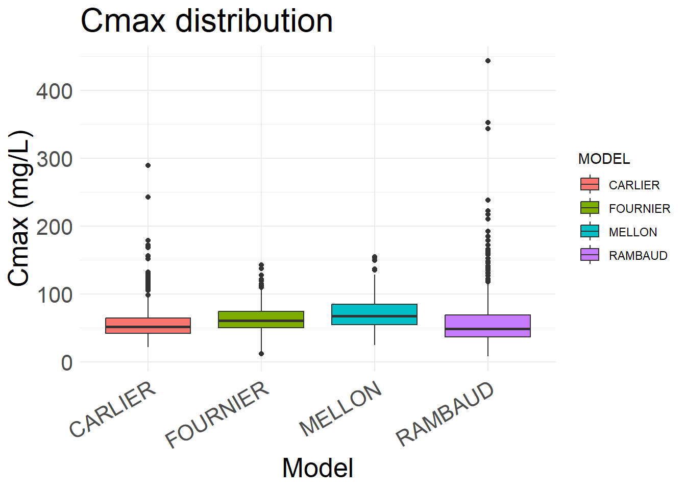
6.4.2 Maximal concentration (Cmax)

Cmax is the true Cmax, not the highest observed concentration.

AMOX_CMAX1 <- all_results %>%
  group_by(ID, MODEL) %>% 
  summarize(
    ID = first(ID),
    MODEL = first(MODEL),
    MODEL_COHORT = first(MODEL_COHORT),
    CMAX_IND = max(Cmax, na.rm = TRUE),  # Cmax based on IPRED
    WT = first(WT), 
    CREAT = first(CREAT), 
    BURN = first(BURN),
    ICU = first(ICU),
    OBESE = first(OBESE),
    AGE = first(AGE),
    SEX = first(SEX),
    HT = first(HT),
    DUR = first(DUR),
    FREQ = first(FREQ),
    DOSE_ADM = first(DOSE_ADM),
    TSS = first(TSS),
    Vc = first(Vc),
    CL = first(CL)
  ) %>%
  mutate(CON = ifelse(DUR == 24, 1, 0))

summarized_CMAX <- AMOX_CMAX1 %>%
  distinct(ID, MODEL, CMAX_IND)

# Box plot for Cmax
plot_CMAX <- ggplot(summarized_CMAX, aes(x = MODEL, y = CMAX_IND, fill = MODEL)) +
  geom_boxplot() +
  theme_minimal() +
  labs(title = "Cmax distribution", x = "Model", y = "Cmax (mg/L)") +
  theme(
    axis.text.x = element_text(angle = 30, hjust = 1),
    axis.text = element_text(size = 16),    
    axis.title = element_text(size = 20), 
    plot.title = element_text(size=24),
  )

plot_CMAX

# Create test data by taking 2400 subjects (24 from each dosing scheme and 6-6 for each model covariate cohorte per dosing scheme)
CMAX_test <- AMOX_CMAX1 %>%
  dplyr::filter(
    ID %% 100 >= 1 & ID %% 100 <= 6 |
      ID %% 100 >= 26 & ID %% 100 <= 31 |
      ID %% 100 >= 51 & ID %% 100 <= 56 |
      ID %% 100 >= 76 & ID %% 100 <= 81
  )

# Create training data by taking 7600 subjects (76 from each dosing scheme and 19-19 for each model covariate cohorte per dosing scheme)
CMAX_train <- AMOX_CMAX1 %>%
  dplyr::filter(
    ID %% 100 >= 7 & ID %% 100 <= 25 |
      ID %% 100 >= 32 & ID %% 100 <= 50 |
      ID %% 100 >= 57 & ID %% 100 <= 75 |
      ID %% 100 >= 82 & ID %% 100 <= 100
  )

# Dataset identifier
CMAX_train_compare <- CMAX_train %>% mutate(Dataset = "Train")
CMAX_test_compare <- CMAX_test %>% mutate(Dataset = "Test")

# Combine the three datasets
combined_CMAX <- bind_rows(CMAX_train_compare, CMAX_test_compare)

# Compare the train and test sets
vars <- c("CREAT", "WT", "CMAX_IND", "CL", "Vc")
tableOne3 <- CreateTableOne(vars = vars, strata = "Dataset", data = combined_CMAX)
tableOne4<-print(tableOne3, nonnormal = c("CREAT", "WT", "CMAX_IND", "CL", "Vc"), printToggle=F, minMax=T)

kableone(tableOne4)

	Test	Train	p	test
n	600	1875
CREAT (median [range])	0.76 [0.24, 5.32]	0.77 [0.13, 8.23]	0.410	nonnorm
WT (median [range])	80.03 [41.33, 139.60]	79.99 [47.36, 141.17]	0.884	nonnorm
CMAX_IND (median [range])	56.16 [13.38, 289.41]	57.91 [8.12, 443.50]	0.138	nonnorm
CL (median [range])	13.08 [0.68, 61.52]	12.70 [1.08, 71.87]	0.462	nonnorm
Vc (median [range])	9.60 [2.17, 38.10]	9.42 [1.73, 51.90]	0.312	nonnorm

Carlier, Mieke, Michaël Noë, Jan J De Waele, Veronique Stove, Alain G Verstraete, Jeffrey Lipman, and Jason A Roberts. 2013. “Population Pharmacokinetics and Dosing Simulations of Amoxicillin/Clavulanic Acid in Critically Ill Patients.” J. Antimicrob. Chemother. 68 (11): 2600–2608.

Fournier, Anne, Sylvain Goutelle, Yok-Ai Que, Philippe Eggimann, Olivier Pantet, Farshid Sadeghipour, Pierre Voirol, and Chantal Csajka. 2018. “Population Pharmacokinetic Study of Amoxicillin-Treated Burn Patients Hospitalized at a Swiss Tertiary-Care Center.” Antimicrobial Agents and Chemotherapy 62 (9): e00505–18. https://doi.org/10.1128/AAC.00505-18.

Mellon, G, K Hammas, C Burdet, X Duval, C Carette, N El-Helali, L Massias, F Mentré, S Czernichow, and A -C Crémieux. 2020. “Population Pharmacokinetics and Dosing Simulations of Amoxicillin in Obese Adults Receiving Co-Amoxiclav.” Journal of Antimicrobial Chemotherapy 75 (12): 3611–18. https://doi.org/10.1093/jac/dkaa368.

Rambaud, Antoine, Benjamin Jean Gaborit, Colin Deschanvres, Paul Le Turnier, Raphaël Lecomte, Nathalie Asseray-Madani, Anne-Gaëlle Leroy, et al. 2020. “Development and Validation of a Dosing Nomogram for Amoxicillin in Infective Endocarditis.” The Journal of Antimicrobial Chemotherapy 75 (10): 2941–50. https://doi.org/10.1093/jac/dkaa232.