4 Validation PKpop Amox Mellon 2020

Show the code

here::i_am("Model_implementation_validation/quarto/valid_amox_mellon_hammas_2020.qmd")
# Functions used for simulation-----

# export functions contained in the "functions" folder
list_of_function_path = list.files(
  path = here::here("Model_implementation_validation/R_functions/"),
  pattern = ".*\\.R$",
  full.names = TRUE
  ) 

purrr::walk(.x=list_of_function_path,.f=source)

5 Paper

Mellon et al. (2020)

Show the code

readr::read_csv(
  file = here::here("Model_implementation_validation/data/mellon_hammas_2020/model_description.csv"),
  show_col_types = F
) |> 
  knitr::kable()

Table 5.1: Model description

DOI	structural_model	variability_model	covariate_effects	patients_number	free_or_total_concentrations	unbound fraction
doi:10.1093/jac/dkaa368	2-comp	interindividual variability for all parameters, log-distribution for all parameters except F	weight on absorption rate	27	total	0.8

5.1 Model parameters

Show the code

# when @correlation is used in OMEGA, mrgsolve assume off-diagonal elements to be correlation coefficients
# and calculate the covariances
# we want to use a single omega matrix, so no correlation matrix will be used
# thus instead of the correlation coefficient between eta CL and ETA Q we have to enter their covariance 
# the following formula is used : 
# covariance(CL, Q) = correlation coefficient(CL,Q)*(SD(CL)*SD(Q))
# SD = standard deviation 

cov_CL_Q = 0.9*(0.27*0.59)
# value rounded to two significant numbers : 0.14

Show the code

readr::read_csv(
  file = here::here("Model_implementation_validation/data/mellon_hammas_2020/model_parameters.csv"),
  show_col_types = F
) |> 
  knitr::kable()

Table 5.2: Model parameters

DOI	parameter_name	parameter_description	unit	mean	rse
10.1093/jac/dkaa368	Fpop	Typical oral bioavailability	unitless	0.797	5
10.1093/jac/dkaa369	Mtt_pop	Typical mean transit time	h	1.000	6
10.1093/jac/dkaa370	Ktr_pop	Typical transit rate	h-1	1.600	11
10.1093/jac/dkaa371	Ka_pop	Typical absorption rate constant	h-1	1.700	10
10.1093/jac/dkaa372	beta_weight	Relation between weight and absorption rate constant	log h-1	-3.100	19
10.1093/jac/dkaa373	CLpop	Typical clearance	L/h	14.600	5
10.1093/jac/dkaa374	Vcpop	Typical central volume of distribution	L	9.000	11
10.1093/jac/dkaa375	Qpop	Typical intercompartimental clearance	L/h	4.200	12
10.1093/jac/dkaa376	Vppop	Typical peripheral volume of distribution	L	6.400	8
10.1093/jac/dkaa377	omega_F	Standard deviation of F random effect	unitless	1.000	20
10.1093/jac/dkaa378	omega_Mtt	Standard deviation of Mtt random effect	unitless	0.250	19
10.1093/jac/dkaa379	omega_Ktr	Standard deviation of Ktr random effect	unitless	0.490	17
10.1093/jac/dkaa380	omega_Ka	Standard deviation of Ka random effect	unitless	0.250	40
10.1093/jac/dkaa381	omega_V1	Standard deviation of V1 random effect	unitless	0.500	17
10.1093/jac/dkaa382	omega_CL	Standard deviation of CL random effect	unitless	0.270	16
10.1093/jac/dkaa383	omega_V2	Standard deviation of V2 random effect	unitless	0.300	23
10.1093/jac/dkaa384	omega_Q	Standard deviation of Q random effect	unitless	0.590	15
10.1093/jac/dkaa385	correlation	Correlation between random effects of CL and Q	unitless	0.900	7
10.1093/jac/dkaa386	SD_a	Standard deviation of the additive component for the residual error model	mg/L	0.383	15
10.1093/jac/dkaa387	SD_b	Standard deviation of the proportional component for the residual error model	mg/L	0.131	7

Given both the concentration’s values and the values of standard deviations of the additive and proportional components of the residual error model for the basic model, we choose to divide by 100 the component’s values announced for the final model with covariates.

5.2 Interindividual variability and covariate effects

The only covariate retained by the article’s authors is weight.

\[ Ka_{i} = Ka_{pop} \times (BW/109.3)^{beta_{weight}} \times exp(\eta^{Ka}) \]

With :

\(Ka_{i}\) : absorption rate for individual i (\(h^{-1}\))
\(BW\) : bodyweight of the individual i (kg)
\(\eta_{Ka}\) : normal variable with mean 0 and variance \({\omega_{Ka}}^2\)

Other parameters defined in Table 5.2.

According to the article, all model parameters are log-normally distributed, except F wich is logit transformed :

\[ F = log(F_{pop}/(1-F_{pop})) + \eta^F \] With :

\(EF\) : normal variable with mean 0 and variance \({\omega_{F}}^2\)

6 Validation of the model implementation

To validate the model’s implementation, simulations were compared with the article’s observations of figure 1 and 3.

For the simulations appearing later in the article, “body weight was randomly drawn from a uniform distribution [85–155 kg], which corresponds to the range of weights observed at the inclusion of participating subjects”. To create “patients” for our simulations, weights were sampled from a uniform distribution with that density.

7 Figure 1

Show the code

# generate weights from the uniform distribution : 
set.seed(100)
weights = runif(n = 27, min = 85, max = 155)|>
  as.data.frame() |>
  dplyr::rename(BW = "runif(n = 27, min = 85, max = 155)") |> 
  dplyr::mutate(ID = 1:27)
write.csv(weights, file = here::here("Model_implementation_validation/data/mellon_hammas_2020/patients_weights.csv"), row.names = FALSE)

First, we created 27 “patients” by sampling weights from the uniform distribution described above. We then simulated concentrations for 27 “patients” using typical parameters values and inter individual variability. This was intended as a control.

The weights of the patients included in the study are unknown. Moreover, our simulations were taking inter individual variability in account. As a result, we were not expecting to reproduce the observed concentrations profiles described in figure 1. This was intended as a control of the overall time-concentration profile.

Show the code

# in the article, "An ‘IV + oral obese population PK model’ was then adjusted to the whole set  
# of amoxicillin concentration data obtained after both IV and oral administration."
# Our model has to be used for oral and IV simulations. 

# simulations for 27 patients, oral administration : 

# arguments : 

# dosing regimen
dose_oral = readr::read_csv(file = here::here("Model_implementation_validation/data/mellon_hammas_2020/dosing_regimen.csv"), show_col_types = F) |>
  dplyr::filter(regimen_id == "oral") |> mrgsolve::as.ev()
dose_oral

sim_dur_8h = 8

model = mrgsolve::mread(model = here::here("Model_implementation_validation/mrgsolve/amox_Mellon.cpp"),show_col_types = F)

patients = read.csv(file = here::here("Model_implementation_validation/data/mellon_hammas_2020/patients_weights.csv")) 
patients

sim_step = 1/6

path_to_param = here::here("Model_implementation_validation/data/mellon_hammas_2020/model_parameters.csv")

default = list(MIC = 1, BW = 1)

# simulation : 
sim_oral_8h_27_patients = simulate_mrgsolve(dosing_regimen = dose_oral,
                                            sim_dur = sim_dur_8h,
                                            model = model,
                                            patients = patients,
                                            sim_step = sim_step,
                                            param_file = path_to_param,
                                            cov_default = default,
                                            omega_mat = NULL)
sim_oral_8h_27_patients


# simulations for 27 patients, one infusion of 60 minutes
# dosing in the second compartment (CENTRAL)

# dose
dose_iv = readr::read_csv(file = here::here("Model_implementation_validation/data/mellon_hammas_2020/dosing_regimen.csv"), show_col_types = F) |>
  dplyr::filter(regimen_id=="IV") |>
  mrgsolve::as.ev()
dose_iv

# simulation
sim_iv_8h_27_patients = simulate_mrgsolve(dosing_regimen = dose_iv,
                                            sim_dur = sim_dur_8h,
                                            model = model,
                                            patients = patients,
                                            sim_step = sim_step,
                                            param_file = path_to_param,
                                            cov_default = default,
                                            omega_mat = NULL)
sim_iv_8h_27_patients

Show the code

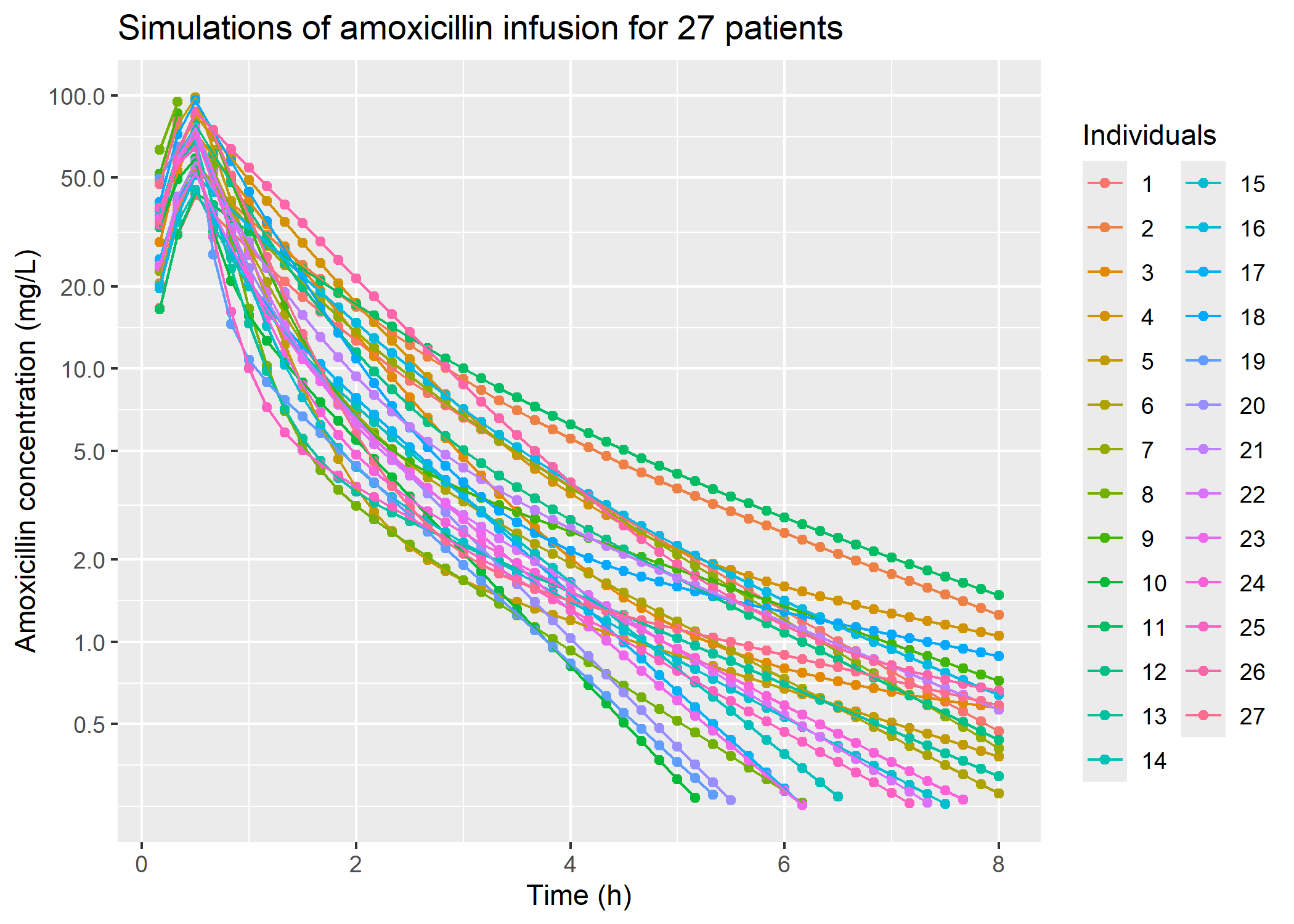
# plot IV administration
plot_iv_8h_27_patients = sim_iv_8h_27_patients |> 
  dplyr::filter(time != 0) |>
  ggplot2::ggplot(mapping = ggplot2::aes(x = time, y = IPRED, color = as.factor(ID))) + 
  ggplot2::geom_point() +
  ggplot2::geom_line() +
  ggplot2::scale_y_continuous(transform = "log2",
                              breaks = c(0.5, 1, 2, 5, 10, 20, 50, 100),
                              limits = c(0.25, 100)) +
  ggplot2::labs(title = "Simulations of amoxicillin infusion for 27 patients",
                color = "Individuals",
                y = "Amoxicillin concentration (mg/L)",
                x = "Time (h)")
plot_iv_8h_27_patients

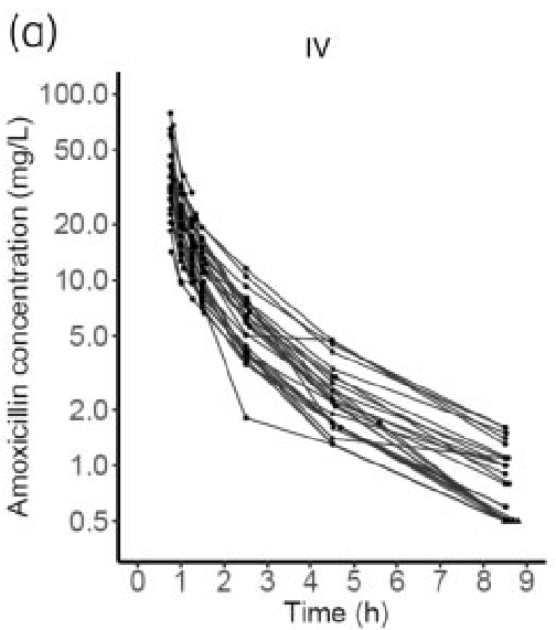
Article’s figure 1a, IV administration, compared with simulations

For amoxicillin IV administration, Cmax and the most of the time-concentration profiles look similar. However, for a lot of the simulated “patients” concentrations decrease quicker or to lower values than the real patient’s of the article.

Show the code

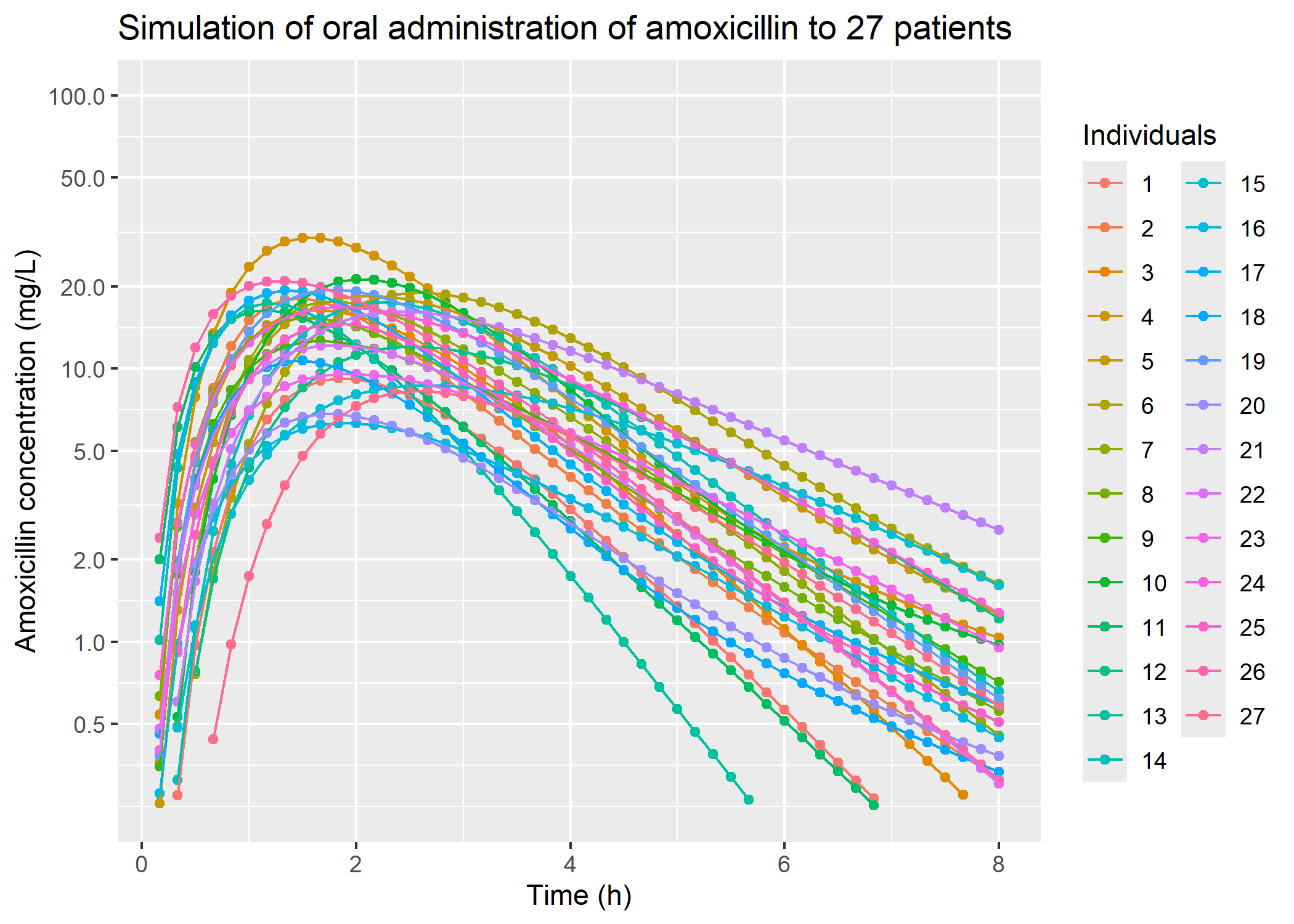
# plot oral administration: 
plot_oral_8h_27_patients = sim_oral_8h_27_patients |> 
  dplyr::filter(time != 0) |>
  ggplot2::ggplot(mapping = ggplot2::aes(x = time, y = IPRED, color = as.factor(ID))) + 
  ggplot2::geom_point() +
  ggplot2::geom_line() +
  ggplot2::scale_y_continuous(transform = "log2",
                              breaks = c(0.5, 1, 2, 5, 10, 20, 50, 100),
                              limits = c(0.25, 100)) +
  ggplot2::labs(title = "Simulation of oral administration of amoxicillin to 27 patients",
                color = "Individuals",
                y = "Amoxicillin concentration (mg/L)",
                x = "Time (h)")
plot_oral_8h_27_patients

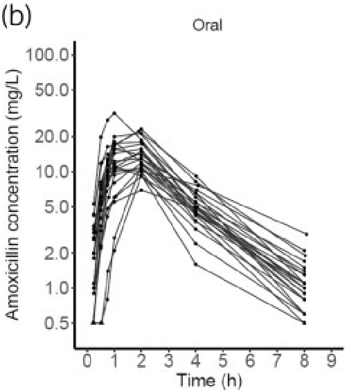
Article’s figure 1b, oral administration, compared with simulations

For amoxicillin oral administration, Tmax and Cmax of our simulations and the original article looks the same and overall profile seems similar. However, like for IV administration, some simulated patients’ concentrations decrease more and quicker than the real patients’.

Those differences may be caused by interindividual variability and differences between real and simulate dpatients’ weights.

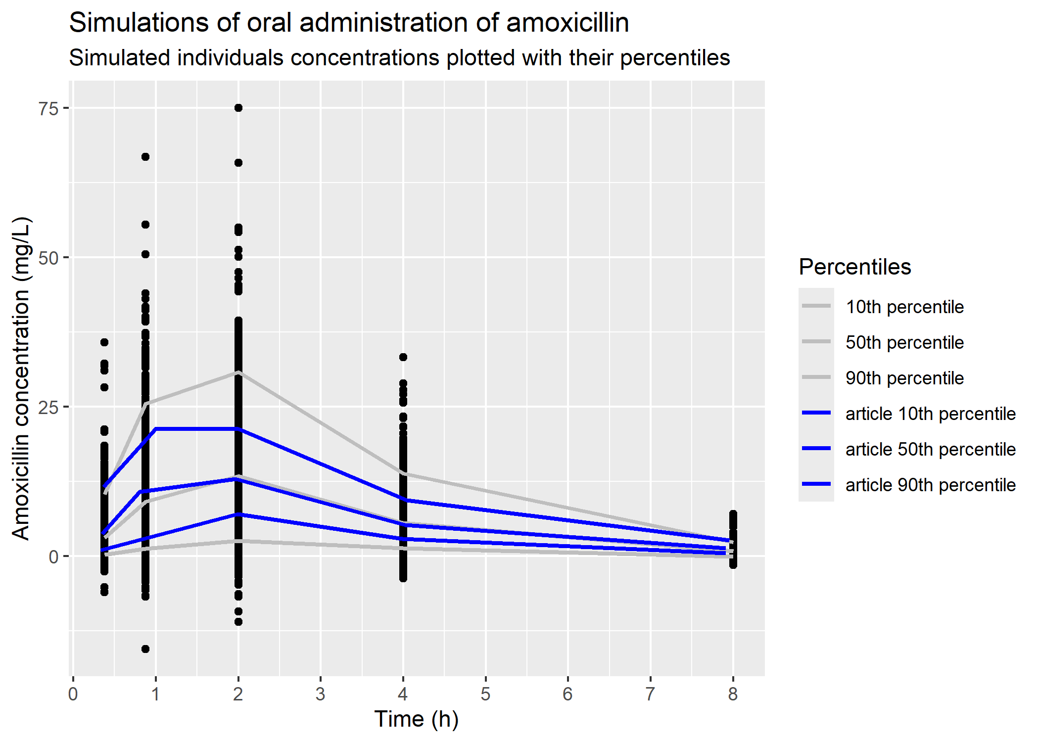
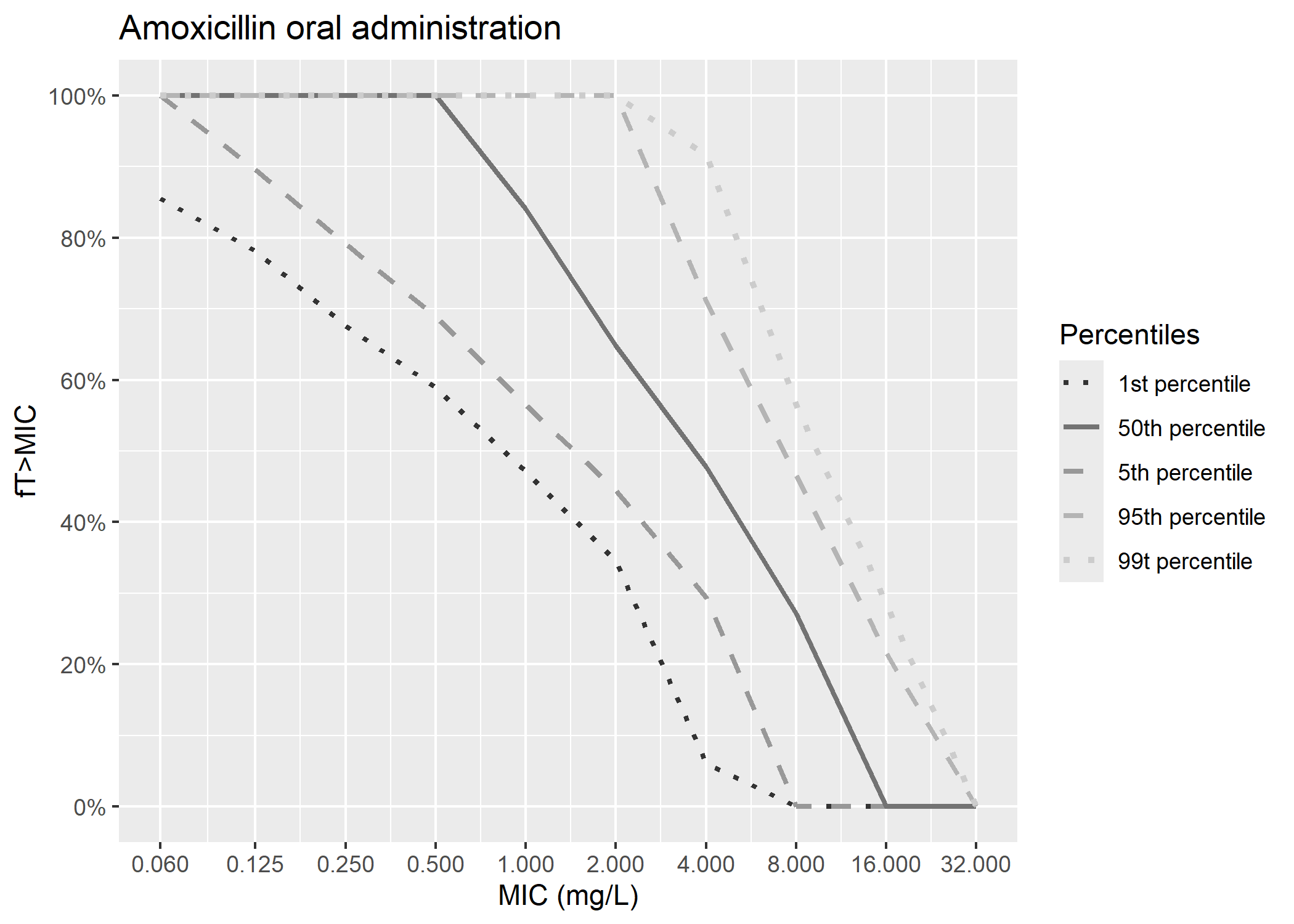
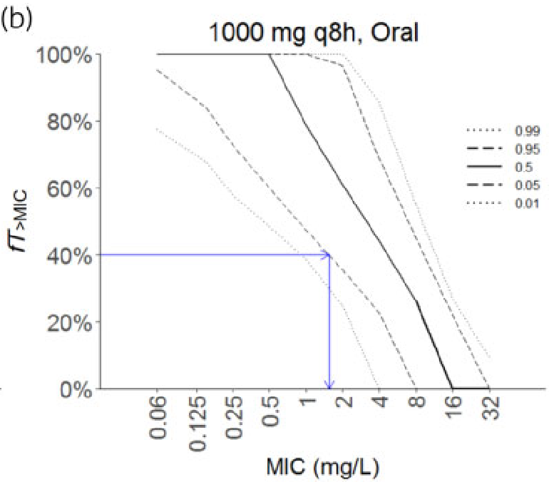
8 Figure 3

In the article, 500 simulations were used in order to generate visual predictive check (VPC) for the final model. We simulated 500 “patients” with different weights to reproduce figure 3.

Show the code

# generate weights from the uniform distribution : 
set.seed(100)
weights_500 = runif(n = 500, min = 85, max = 155)|>
  as.data.frame() |>
  dplyr::rename(BW = "runif(n = 500, min = 85, max = 155)") |> 
  dplyr::mutate(ID = 1:500)
write.csv(weights_500, file = here::here("Model_implementation_validation/data/mellon_hammas_2020/patients_weights_500.csv"), row.names = FALSE)

According to the article, amoxicillin plasmatic concentration measurements were done before administration and 15, 30, 45, 60, 120, 240 and 480 minutes after. Given these facts and figure 3, it looks like 5 bins were done to compute VPCs for amoxicillin oral administration : between 15 and 30 minutes, between 45 and 60 minutes, at 2, 4 and 8 hours. We tried to reproduce that binning.

We plotted 10th, 50th and 90th percentiles of our simulations with the corresponding percentiles of the siulations in figure 3. Percentiles of the simulation were retrieved from the article’s figures by digitizing the middle of the 95% confidence interval of the simulations.

Show the code

# 5 bins observées sur le graphique
# rappeler temps de prélèvements indiqués dans l'article # infos sur reproduction figure 
# mimer le binning 
# mais écart normal et attendu 

sim_dur_8h = 8

model = mrgsolve::mread(model = here::here("Model_implementation_validation/mrgsolve/amox_Mellon.cpp"),show_col_types = F)

five_hundreds_patients = read.csv(file = here::here("Model_implementation_validation/data/mellon_hammas_2020/patients_weights_500.csv"))
five_hundreds_patients

sim_step_quarter = 1/4

path_to_param = here::here("Model_implementation_validation/data/mellon_hammas_2020/model_parameters.csv")

default = list(MIC = 1, BW = 1)

# simulation
# créer un vecteur avec les temps utilisés pour les bins 


# filter time in... (pour avoir simulations aux temps de prélèvement)
# créer une colonne milieu de bin (bin_mid) --> case_when : si temps à 15 ou 30 : valeur 22, 5 
# (médiane temps du bin, prendre la moy par convention) --> faire la moyenne 
# idem pour 45 et 60 min 
# 2, 4, et 8h prendre directement les tmeps

vec_selected_times <- c(0.25, 0.50, 0.75, 1, 2, 4, 8)


#sim_iv_500_patients |>
#  dplyr::mutate(bin_mid = dplyr::case_when(time %in% c(0.25, 0.5) ~ 0.375,
#                                           time %in% c(0.75, 1) ~ 0.875))
# valeur <- dplyr::case_when(sim_iv_500_patients_3$time %in% c(0,2) ~ "super")


# mean 0.25 and 0.5 : 0.375
# mean 0.75 and 1 : 0.875



# per os
dose_oral = readr::read_csv(file = here::here("Model_implementation_validation/data/mellon_hammas_2020/dosing_regimen.csv"), show_col_types = F) |>
  dplyr::filter(regimen_id == "oral") |> mrgsolve::as.ev()
dose_oral

sim_oral_500_patients = simulate_mrgsolve(dosing_regimen = dose_oral,
                                            sim_dur = sim_dur_8h,
                                            model = model,
                                            patients = five_hundreds_patients,
                                            sim_step = sim_step,
                                            param_file = path_to_param,
                                            cov_default = default,
                                            omega_mat = NULL)|>
  dplyr::filter(time %in% vec_selected_times) |>
  dplyr::select(ID, time, Y)
sim_oral_500_patients

# mean 0.25 and 0.5 : 0.375
# mean 0.75 and 1 : 0.875

first_bin_oral = sim_oral_500_patients |>
  dplyr::filter(time %in%c(0.25,0.50)) |>
  dplyr::group_by(ID) |>
  dplyr::summarise(mean_CP = mean(Y)) |>
  dplyr::mutate(time = 0.375) |>
  dplyr::rename(Y = mean_CP)
first_bin_oral

second_bin_oral = sim_oral_500_patients |>
  dplyr::filter(time %in%c(0.75, 1)) |>
  dplyr::group_by(ID) |>
  dplyr::summarise(mean_CP = mean(Y)) |>
  dplyr::mutate(time = 0.875) |>
  dplyr::rename(Y = mean_CP)
second_bin_oral

other_bins_oral = sim_oral_500_patients |>
  dplyr::filter(time %in% c(2, 4, 8)) |>
  dplyr::relocate(ID, Y)
other_bins_oral

sim_oral_500_patients_for_plot = dplyr::full_join(x = first_bin_oral, y = second_bin_oral) |>
  dplyr::full_join(y = other_bins_oral)
sim_oral_500_patients_for_plot

Show the code

# oral administration


# article data
fig_3b_10_percentile = readr::read_csv(here::here("Model_implementation_validation/data/mellon_hammas_2020/fig_article/percentiles_simulation/fig_3_b_p10th_sim.csv"), show_col_types = F) 

fig_3b_50_percentile = readr::read_csv(here::here("Model_implementation_validation/data/mellon_hammas_2020/fig_article/percentiles_simulation/fig_3_b_p50th_sim.csv")) 

fig_3b_90_percentile = readr::read_csv(here::here("Model_implementation_validation/data/mellon_hammas_2020/fig_article/percentiles_simulation/fig_3_b_p90th_sim.csv"), show_col_types = F) 


# plot
plot_sim_oral_500_patients_points = sim_oral_500_patients_for_plot |>
  dplyr::summarise(
    .by = time,
    q10 = quantile(Y, 0.10),
    q50 = quantile(Y, 0.5),
    q90 = quantile(Y, 0.90)
  ) |>
  ggplot2::ggplot() +
  ggplot2::geom_point(data = sim_oral_500_patients_for_plot, mapping = ggplot2::aes(x = time, y = Y)) +
  ggplot2::geom_line(mapping = ggplot2::aes(x = time, y = q10, color = "10th percentile"), 
                     linewidth = 1) +
  ggplot2::geom_line(mapping = ggplot2::aes(x = time, y = q50, color = "50th percentile"), 
                     linewidth = 1) + 
  ggplot2::geom_line(mapping = ggplot2::aes(x = time, y = q90, color = "90th percentile"), 
                     linewidth = 1) +
  ggplot2::geom_line(data = fig_3b_10_percentile, mapping = ggplot2::aes(x = time, y = CP, color = "article 10th percentile"),
                                                         linewidth = 1) +
  
  ggplot2::geom_line(data = fig_3b_50_percentile, mapping = ggplot2::aes(x = time, y = CP, color = "article 50th percentile"),
                                                         linewidth = 1) +
  
  ggplot2::geom_line(data = fig_3b_90_percentile, mapping = ggplot2::aes(x = time, y = CP, color = "article 90th percentile"),
                                                         linewidth = 1) +
  ggplot2::scale_color_manual(values = c("grey", "grey", "grey","blue", "blue", "blue")) +
  ggplot2::scale_x_continuous(breaks = c(0, 1, 2, 3, 4, 5, 6, 7, 8, 9)) +
  ggplot2::labs(title = "Simulations of oral administration of amoxicillin", 
                subtitle = "Simulated individuals concentrations plotted with their percentiles", 
                colour = "Percentiles",
                x = "Time (h)",
                y = "Amoxicillin concentration (mg/L)")
plot_sim_oral_500_patients_points

The median of our simulations line up quite well with what was found in the paper. There is more variability in our simulation than in the paper but this could be attributed to a different distribution of patient weights in the real dataset, indeed we simulated using a uniform distribution between the minimum and maximum weights reported in the paper while it would be plausible that the real weights were more concentrated towards the center of the distribution. Also the binning will impact the closeness of our simulations with the published VPC.

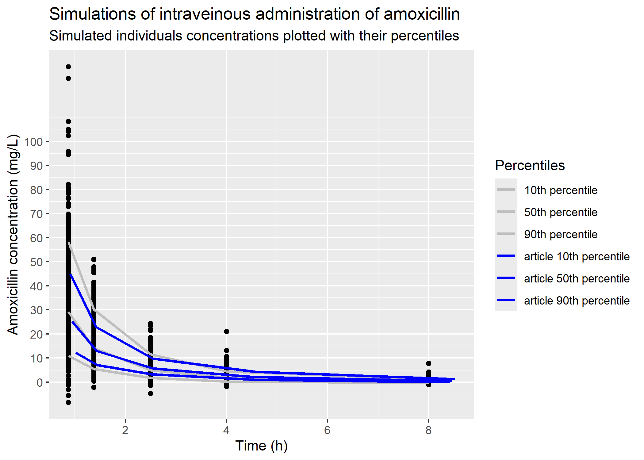
Total concentrations :

Show the code

# bins may differ between IV and oral administration
# It looks like there are 5 bins : between 45 minutes and 1 hour, 1 and two hour, 2 and 3 hours, 4 hours, 8 hours 

# dosing regimen
dose_iv = readr::read_csv(file = here::here("Model_implementation_validation/data/mellon_hammas_2020/dosing_regimen.csv"), show_col_types = F) |>
  dplyr::filter(regimen_id=="IV") |>
  mrgsolve::as.ev()
dose_iv

sim_dur_8h = 8

model = mrgsolve::mread(model = here::here("Model_implementation_validation/mrgsolve/amox_Mellon.cpp"),show_col_types = F)

five_hundreds_patients = read.csv(file = here::here("Model_implementation_validation/data/mellon_hammas_2020/patients_weights_500.csv"))
five_hundreds_patients

sim_step_quarter = 1/4

path_to_param = here::here("Model_implementation_validation/data/mellon_hammas_2020/model_parameters.csv")

default = list(MIC = 1, BW = 1)

# in order to use omega matrices default values, omega_mat = NULL

# times needed to create the bins
vec_selected_times_2 <- c(0.75, 1, 1.25, 1.5, 2, 3, 4, 8)

# simulation
sim_iv_500_patients_2 = simulate_mrgsolve(dosing_regimen = dose_iv,
                                            sim_dur = sim_dur_8h,
                                            model = model,
                                            patients = five_hundreds_patients,
                                            sim_step = sim_step_quarter,
                                            param_file = path_to_param,
                                            cov_default = default,
                                            omega_mat = NULL) |>
  dplyr::filter(time %in% vec_selected_times_2) |>
  dplyr::select(ID, time, Y)
sim_iv_500_patients_2

# bins 
first_bin_iv = sim_iv_500_patients_2 |>
  dplyr::filter(time %in%c(0.75,1)) |>
  dplyr::group_by(ID) |>
  dplyr::summarise(mean_CP = mean(Y)) |>
  dplyr::mutate(time = 0.875) |>
  dplyr::rename(Y = mean_CP)
first_bin_iv

second_bin_iv = sim_iv_500_patients_2 |>
  dplyr::filter(time %in%c(1.25, 1.5)) |>
  dplyr::group_by(ID) |>
  dplyr::summarise(mean_CP = mean(Y)) |>
  dplyr::mutate(time = 1.375) |>
  dplyr::rename(Y = mean_CP)
second_bin_iv

third_bin_iv = sim_iv_500_patients_2 |>
  dplyr::filter(time %in%c(2, 3)) |>
  dplyr::group_by(ID) |>
  dplyr::summarise(mean_CP = mean(Y)) |>
  dplyr::mutate(time = 2.5) |>
  dplyr::rename(Y = mean_CP)
third_bin_iv

bins_4_and_5 = sim_iv_500_patients_2 |>
  dplyr::filter(time %in% c(4, 8)) |>
  dplyr::relocate(ID, Y)
bins_4_and_5

# data frame 
sim_iv_500_patients_for_plot_2 = dplyr::full_join(x = first_bin_iv, y = second_bin_iv) |>
  dplyr::full_join(y = third_bin_iv) |>
  dplyr::full_join(y = bins_4_and_5)
sim_iv_500_patients_for_plot_2

Show the code

# article data
fig_3a_10_percentile = readr::read_csv(here::here("Model_implementation_validation/data/mellon_hammas_2020/fig_article/percentiles_simulation/fig_3_a_p10th_sim.csv"), show_col_types = F) 

fig_3a_50_percentile = readr::read_csv(here::here("Model_implementation_validation/data/mellon_hammas_2020/fig_article/percentiles_simulation/fig_3_a_p50th_sim.csv"), show_col_types = F) 

fig_3a_90_percentile = readr::read_csv(here::here("Model_implementation_validation/data/mellon_hammas_2020/fig_article/percentiles_simulation/fig_3_a_p90th_sim.csv"), show_col_types = F) 

# plot
plot_sim_iv_500_patients_points_2 = sim_iv_500_patients_for_plot_2 |>
  dplyr::summarise(
    .by = time,
    q10 = quantile(Y, 0.10),
    q50 = quantile(Y, 0.5),
    q90 = quantile(Y, 0.90)
  ) |>
  ggplot2::ggplot() +
  ggplot2::geom_point(data = sim_iv_500_patients_for_plot_2, mapping = ggplot2::aes(x = time, y = Y)) +
  ggplot2::geom_line(mapping = ggplot2::aes(x = time, y = q10, color = "10th percentile"), 
                     linewidth = 1) +
  ggplot2::geom_line(mapping = ggplot2::aes(x = time, y = q50, color = "50th percentile"), 
                     linewidth = 1) + 
  ggplot2::geom_line(mapping = ggplot2::aes(x = time, y = q90, color = "90th percentile"), 
                     linewidth = 1) + 
  ggplot2::geom_line(data = fig_3a_10_percentile, mapping = ggplot2::aes(x = time, y = CP, color = "article 10th percentile"),
                                                         linewidth = 1) +
  
  ggplot2::geom_line(data = fig_3a_50_percentile, mapping = ggplot2::aes(x = time, y = CP, color = "article 50th percentile"),
                                                         linewidth = 1) +
  
  ggplot2::geom_line(data = fig_3a_90_percentile, mapping = ggplot2::aes(x = time, y = CP, color = "article 90th percentile"),
                                                         linewidth = 1) +
  ggplot2::scale_y_continuous(breaks = c(0, 10, 20, 30, 40, 50, 60, 70, 80, 90, 100)) +
  ggplot2::scale_color_manual(values = c("grey", "grey", "grey","blue", "blue", "blue")) +
  ggplot2::labs(title = "Simulations of intraveinous administration of amoxicillin", 
                subtitle = "Simulated individuals concentrations plotted with their percentiles", 
                colour = "Percentiles",
                x = "Time (h)",
                y = "Amoxicillin concentration (mg/L)") 
plot_sim_iv_500_patients_points_2

Overall our simulations line up quite well with what was found in the paper. Slight differences were expected due to binning.

9 Figure 4

Show the code

# generate weights from the uniform distribution : 
set.seed(100)
weights_1000 = runif(n = 1000, min = 85, max = 155) |>
  as.data.frame() |>
  dplyr::rename(BW = "runif(n = 1000, min = 85, max = 155)") |> 
  dplyr::mutate(ID = 1:1000)

write.csv(weights_1000, file = here::here("Model_implementation_validation/data/mellon_hammas_2020/patients_weights_1000.csv"), row.names = FALSE)

Show the code

ft_over_mic = function(dosing_regimen, sim_dur, model, patients, sim_step,
           param_file, cov_default, omega_mat, from, to) {
  
  sim_tbl = simulate_mrgsolve(dosing_regimen, sim_dur, model, patients, sim_step,
           param_file, cov_default, omega_mat)
  
  ft_over_mic = sim_tbl |>
    compute_ft_over_mic(from, to) |>
    dplyr::ungroup()
}

all_mics_ft_over_mic = function(dosing_regimen, sim_dur, model, patients, sim_step,
           param_file, weigth, omega_mat, from, to) {
  all_tibbles = purrr::map(mics,~ft_over_mic(dosing_regimen, sim_dur, model, patients, sim_step,
           param_file, cov_default = list(MIC = .x, BW = weigth), omega_mat, from, to)) 
  
  purrr::map(all_tibbles,~as.data.frame(x = .x)) |>
    dplyr::bind_rows()
}

Show the code

# 30 minutes IV infusion 3 times daily : 
path_dosing_regimens = here::here("Model_implementation_validation/data/mellon_hammas_2020/dosing_regimen.csv")
iv_1g_q8h = select_dosing_regimens(selected_regimens = list("IV 1000 mg q8h"),
                                   path_to_the_file = path_dosing_regimens)
iv_1g_q8h

sim_dur_48 = 48

model = mrgsolve::mread(model = here::here("Model_implementation_validation/mrgsolve/amox_Mellon.cpp"),show_col_types = F)

one_thousand_patients = read.csv(file = here::here("Model_implementation_validation/data/mellon_hammas_2020/patients_weights_1000.csv"))
one_thousand_patients

sim_step = 1/6

path_to_param = here::here("Model_implementation_validation/data/mellon_hammas_2020/model_parameters.csv")

default = list(MIC = 1, BW = 1)

# in order to use omega matrices default values : 
null_matrices = list(diag_iiv = mrgsolve::dmat(numeric(6)), corr_iiv = mrgsolve::bmat(numeric(3)))

sim_iv_1000_patients = simulate_mrgsolve(dosing_regimen = iv_1g_q8h,
                                            sim_dur = sim_dur_48,
                                            model = model,
                                            patients = one_thousand_patients,
                                            sim_step = sim_step,
                                            param_file = path_to_param,
                                            cov_default = default,
                                            omega_mat = null_matrices)
sim_iv_1000_patients

mics = list(0.06, 0.125, 0.25, 0.5, 1, 2, 4, 8, 16, 32)
mics

ft_over_mic_iv = ft_over_mic(dosing_regimen = iv_1g_q8h,
                             sim_dur = sim_dur_48,
                             model = model,
                             patients = one_thousand_patients,
                             sim_step = sim_step,
                             param_file = path_to_param,
                             cov_default = default,
                             omega_mat = null_matrices,
                             from = 24,
                             to = 48)  
ft_over_mic_iv

set.seed(1000)
all_mics_iv = all_mics_ft_over_mic(dosing_regimen = iv_1g_q8h,
                             sim_dur = sim_dur_48,
                             model = model,
                             patients = one_thousand_patients,
                             sim_step = sim_step,
                             param_file = path_to_param,
                             weigth = 1,
                             omega_mat = null_matrices,
                             from = 24,
                             to = 48)
all_mics_iv 

write.csv(all_mics_iv, file = here::here("Model_implementation_validation/data/mellon_hammas_2020/results/all_ft_over_mics_iv.csv"))


# 1g 3 times daily per os 

oral_1g_q8h = select_dosing_regimens(selected_regimens = list("oral 1000 mg q8h"),
                                     path_to_the_file = path_dosing_regimens)
oral_1g_q8h


all_mics_oral = all_mics_ft_over_mic(dosing_regimen = oral_1g_q8h,
                             sim_dur = sim_dur_48,
                             model = model,
                             patients = one_thousand_patients,
                             sim_step = sim_step,
                             param_file = path_to_param,
                             weigth = 1,
                             omega_mat = null_matrices,
                             from = 24,
                             to = 48)
all_mics_oral

write.csv(all_mics_oral, file = here::here("Model_implementation_validation/data/mellon_hammas_2020/results/all_ft_over_mics_oral.csv"))

sim_oral_1000_patients = simulate_mrgsolve(dosing_regimen = oral_1g_q8h,
                                            sim_dur = sim_dur_48,
                                            model = model,
                                            patients = one_thousand_patients,
                                            sim_step = sim_step,
                                            param_file = path_to_param,
                                            cov_default = default,
                                            omega_mat = null_matrices)
sim_oral_1000_patients

Show the code

# plot IV
plot_iv_fig_4 = all_mics_iv |>
  dplyr::summarise(
    .by = MIC,
    q01 = quantile(ft_over_mic, 0.01),
    q05 = quantile(ft_over_mic, 0.05),
    q50 = quantile(ft_over_mic, 0.5),
    q95 = quantile(ft_over_mic, 0.95),
    q99 = quantile(ft_over_mic, 0.99)
  ) |>
  ggplot2::ggplot(mapping = ggplot2::aes(y = ft_over_mic)) +
  ggplot2::scale_x_continuous(name = "MIC (mg/L)", transform = "log2",
      breaks = c(0.06, 0.125, 0.25, 0.5, 1, 2, 4, 8, 16, 32)) +
  ggplot2::scale_y_continuous(name = "fT>MIC", breaks = c(0, 0.2, 0.4, 0.6, 0.8, 1),
                              labels = c("0%", "20%", "40%", "60%", "80%", "100%")) +
  ggplot2::geom_line(mapping = ggplot2::aes(x = MIC, y = q01, color = "1st percentile"), 
                     linetype = "dotted",
                     linewidth = 1) +
  ggplot2::geom_line(mapping = ggplot2::aes(x = MIC, y = q05, color = "5th percentile"), 
                     linetype = "dashed",
                     linewidth = 1) + 
  ggplot2::geom_line(mapping = ggplot2::aes(x = MIC, y = q50, color = "50th percentile"), 
                     linewidth = 1) + 
  ggplot2::geom_line(mapping = ggplot2::aes(x = MIC, y = q95, color = "95th percentile"), 
                     linetype = "dashed",
                     linewidth = 1) + 
  ggplot2::geom_line(mapping = ggplot2::aes(x = MIC, y = q99, color = "99th percentile"), 
                     linetype = "dotted",
                     linewidth = 1.2) +
  ggplot2::scale_color_grey() +
  ggplot2::labs(title = "Amoxicillin infusion",
                color = "Percentiles")

plot_iv_fig_4

Our simulations seems to match figure 4 well.