1  Validation PKpop Amox Carlier 2013

Show the code
here::i_am("Model_implementation_validation/quarto/valid_amox_carlier_2013.qmd")
# Functions used for simulation-----

# export functions contained in the "functions" folder
list_of_function_path = list.files(
  path = here::here("Model_implementation_validation/R_functions/"),
  pattern = ".*\\.R$",
  full.names = TRUE
  ) 

purrr::walk(.x=list_of_function_path,.f=source)

2 Paper

(Carlier et al. 2013)

3 Model description

The same model describe both amoxicillin and clavulanic acid concentrations.

Show the code
readr::read_csv(
  file = here::here("Model_implementation_validation/data/carlier_2013/model_description.csv"),
  show_col_types = FALSE 
) |> 
  dplyr::rename("Structural model" = structural_model,
                "Variability model" = variability_model,
                "Covariates effects" = covariate_effects,
                "Number of patients" = patients_number,
                "Free or total concentrations" = free_or_total_concentrations,
                "Unbound fraction" = unbound_fraction) |>
  knitr::kable()
Table 3.1: Model description
DOI Structural model Variability model Covariates effects Number of patients Free or total concentrations Unbound fraction
10.1093/jac/dkt240 2-comp log-normal clearance creatinine clearance on clearance 13 free 0.83

3.1 Model parameters

Show the code
readr::read_csv(
  file = here::here("Model_implementation_validation/data/carlier_2013/model_parameters.csv"),
  show_col_types = F
) |>  
  dplyr::select(-DOI) |> 
  knitr::kable()
Table 3.2: Model parameters for amoxicillin
parameter_name parameter_description unit mean
CLpop Typical clearance (for a patient with creatinin clearance of 102 mL/min) L/h 10.0
Q Intercompartmental clearance L/h 15.6
Vcpop Typical central volume of distribution (for a patient with creatinin clearance of 102 mL/min) L 13.7
Vp Peripheral volume of distribution L 13.7
cv_iiv_CL Coefficient of variation of the inter individual variability on clearance (%) unitless 39.9
cv_iiv_Vc Coefficient of variation of the inter individual variability on central volume of distribution (%) unitless 38.7
ruv Coefficient of variation of the residual variability unitless 22.0

3.2 Inter-individual variability and covariate effects

Covariate effect : \[ TVCL_{i} = CLpop*\frac{CLCR_{i}}{102}*e^{\eta_{i}} \] With :
\(TVCL_{i}\) : Amoxicillin clearance for individual i
\(CLpop\) : Typical amoxicillin clearance (L/h)
\(CLCR_{i}\) : 24h urinary creatinin clearance (mL/min) for individual i
\(\eta_{i}\) : Normal variable with mean 0 and variance \(\omega^2_{CL}\)
\(102\) : population’s median urinary creatinine clearance in mL/min

4 Validation of the mrgsolve implementation of the amoxicillin model

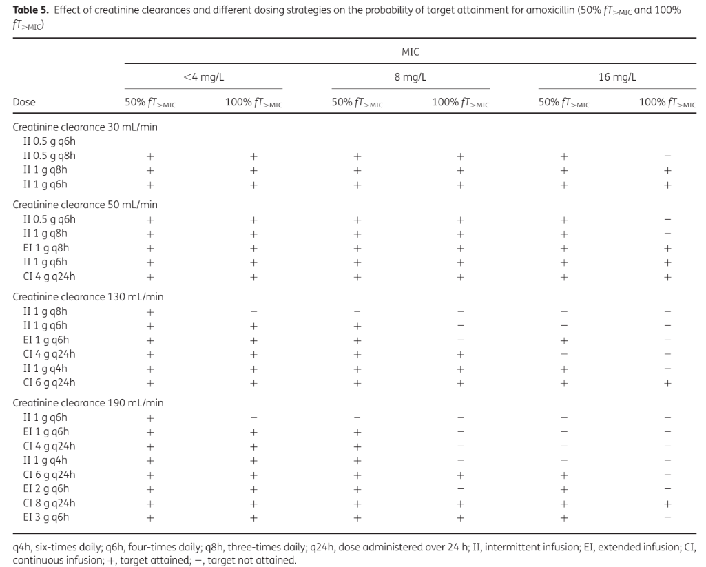
To validate that our implementation of the model is correct we will attempt to reproduce figure 2 and table 5 of the original article.

4.1 Preliminary testing

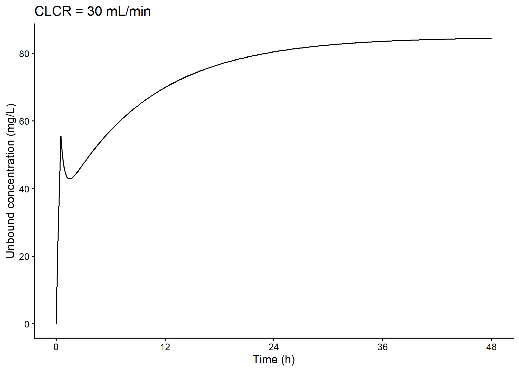
First we check that simulations for a single dosing regimen and creatinine clearance value make sense.

Show the code
path_dosing_regimens = here::here("Model_implementation_validation/data/carlier_2013/dosing_regimen_table_amox.csv")

path_parameters = here::here("Model_implementation_validation/data/carlier_2013/model_parameters.csv")

model = mrgsolve::mread(model = here::here("Model_implementation_validation/mrgsolve/amox_carlier.cpp"))

dosing_reg_6g_q24h = select_dosing_regimens(selected_regimen = "ci 6g q24h",
                              path_to_the_file = path_dosing_regimens)

patients = tibble::tibble(ID = 1)

sim_dur = 48 #hours
sim_step = 1/6 #1 every 10 min
omega_mat = mrgsolve::dmat(0,0)
cov_default = list(MIC = 4,SEX = 0, AGE = 60, BSA = 1.73,CREAT = 2.24)

# simulation for a patient with CLCR = 30 mL/min dosing regimen ci 6g q24h
sim_6g_q24h_clcr_30 <- simulate_mrgsolve(
  dosing_regimen = dosing_reg_6g_q24h,
  sim_dur = sim_dur,
  model = model,
  patients = patients,
  sim_step = sim_step,
  param_file = path_parameters,
  cov_default = cov_default,
  omega_mat = omega_mat)

plot_sim_6g_q24h_clcr_30 = sim_6g_q24h_clcr_30 |> 
  ggplot2::ggplot(mapping = ggplot2::aes(x=time)) + 
  ggplot2::geom_line(mapping=ggplot2::aes(y=IPRED)) + 
  ggplot2::scale_x_continuous(name = "Time (h)",
                              breaks = seq(0,sim_dur,by=12)) + 
  ggplot2::scale_y_continuous(name = "Unbound concentration (mg/L)")+
  ggplot2::theme_classic()+
  ggplot2::ggtitle(label = paste0("CLCR = 30 mL/min"))

plot_sim_6g_q24h_clcr_30

Show the code
pta_ft_over_mic_6g_q24h_clcr_30_MIC_4 = compute_ft_over_mic(
  sim_tbl = sim_6g_q24h_clcr_30,
  from = 24,
  to = 48) |> 
  compute_pta_t_over_mic(target = 0.5)

pta_ft_over_mic_6g_q24h_clcr_30_MIC_4 |> 
  knitr::kable()
MIC mean_ft_over_mic sd_ft_over_mic median_ft_over_mic PTA_0.5
4 1 NA 1 1

Looks ok

4.2 Table 5

This table indicate wether the target is attained for a typical patient receiving amoxicillin, for various dosing regimen and various creatinin clearances.

Show the code
readr::read_csv(path_dosing_regimens, show_col_types = FALSE) |>
  dplyr::rename("Dose (mg)" = amt,
                "Interdose interval (h)" = ii,
                "Infusion duration (h)" = tinf, 
                "Dose regimen" = regimen_id,
                "Loading dose ? " = loading_dose,
                "Infusion type" = infusion_type) |>
  knitr::kable()
Table 4.1: Simulated dosing regimen
Infusion type Loading dose ? Dose regimen time Infusion duration (h) Dose (mg) Interdose interval (h) ss evid cmt
intermittent no ii 0.5g q4h 0.0 0.5 500 4 0 1 1
intermittent no ii 0.5g q6h 0.0 0.5 500 6 0 1 1
intermittent no ii 0.5g q8h 0.0 0.5 500 8 0 1 1
intermittent no ii 1g q4h 0.0 0.5 1000 4 0 1 1
intermittent no ii 1g q6h 0.0 0.5 1000 6 0 1 1
intermittent no ii 1g q8h 0.0 0.5 1000 8 0 1 1
intermittent no ii 2g q6h 0.0 0.5 2000 6 0 1 1
intermittent no ii 2g q8h 0.0 0.5 2000 8 0 1 1
extended no ei 0.5g q4h 0.0 2.0 500 4 0 1 1
extended no ei 0.5g q6h 0.0 3.0 500 6 0 1 1
extended no ei 0.5g q8h 0.0 4.0 500 8 0 1 1
extended no ei 1g q4h 0.0 2.0 1000 4 0 1 1
extended no ei 1g q6h 0.0 3.0 1000 6 0 1 1
extended no ei 1g q8h 0.0 4.0 1000 8 0 1 1
extended no ei 2g q6h 0.0 3.0 2000 6 0 1 1
extended no ei 2g q8h 0.0 4.0 2000 8 0 1 1
extended no ei 3g q6h 0.0 3.0 3000 6 0 1 1
continuous yes 1g over 0.5h ci 6g q24h 0.0 0.5 1000 0 0 1 1
continuous yes 1g over 0.5h ci 6g q24h 0.5 24.0 6000 24 0 1 1
continuous yes 1g over 0.5h ci 4g q24h 0.0 0.5 1000 0 0 1 1
continuous yes 1g over 0.5h ci 4g q24h 0.5 24.0 4000 24 0 1 1
continuous yes 1g over 0.5h ci 3g q24h 0.0 0.5 1000 0 0 1 1
continuous yes 1g over 0.5h ci 3g q24h 0.5 24.0 3000 24 0 1 1
continuous yes 1g over 0.5h ci 8g q24h 0.0 0.5 1000 0 0 1 1
continuous yes 1g over 0.5h ci 8g q24h 0.5 24.0 8000 24 0 1 1
continuous yes 1g over 0.5h ci 12g q24h 0.0 0.5 1000 0 0 1 1
continuous yes 1g over 0.5h ci 12g q24h 0.5 24.0 12000 24 0 1 1
Show the code
convert_clcr_to_creat_mdrd <- function(clcr,
                                  sex = 0,
                                  bsa = 1.73,
                                  age = 60) {
  sex_factor <-  ifelse(sex==0, 1, 0.742)
  creat <-  (clcr / (175 * (age^-0.203) * sex_factor * (bsa / 1.73)))^(-1 /
                                                                         1.154)
  creat
}
clcr_values <- c(30,50,130,190)
creat_values <- convert_clcr_to_creat_mdrd(clcr_values) #convert using mdrd assuming male, 60 yo, and base size

pretty_clcr_values <- paste0(clcr_values," mL/min")

Simulations were performed for 4 creatinine clearance values (30 mL/min, 50 mL/min, 130 mL/min, 190 mL/min).

Show the code
pkpd_targets <- c(0.5,1)
mics <- c(4,8,16)

pretty_pkpd_targets <- paste0(pkpd_targets*100,"%")

Two different fT>MIC were studied (50%, 100%) They were computed for a range of MICs (4, 8, 16 mg/L).

First, \(fT>MIC\) was calculated at steady state. Amoxicillin concentrations were considered at steady state after nine days.

Show the code
table_5_pta_results_path <-
  here::here(
    "Model_implementation_validation/data/carlier_2013/sim_results/table_5_pta_results.csv"
  )

#run only if results does not exist yet
if (!file.exists(table_5_pta_results_path)) {
  #Function to #compute PTA for  1 dosing regimen, 1 CLCR, 1 MIC, enables looping through them
  wrapper_compute_pta <- function(dosing_reg_id,
                                  path_dosing_regimens,
                                  sim_dur,
                                  sim_step,
                                  model,
                                  patients,
                                  path_parameters,
                                  cov_default,
                                  omega_mat,
                                  from,
                                  to,
                                  targets) {
    dosing_reg = select_dosing_regimens(selected_regimen = dosing_reg_id,
                                        path_to_the_file = path_dosing_regimens)
    
    sim <- simulate_mrgsolve(
      dosing_regimen = dosing_reg,
      sim_dur = sim_dur,
      model = model,
      patients = patients,
      sim_step = sim_step,
      param_file = path_parameters,
      cov_default = cov_default,
      omega_mat = omega_mat
    ) |> 
      dplyr::rename(CLCR = CRCL)
    
    pta =
      purrr::map(
        targets,
        
        ~ compute_ft_over_mic(
          sim_tbl = sim,
          from = from,
          to = to
        ) |>
          compute_pta_t_over_mic(target = .x)
      ) |>
      purrr::reduce(dplyr::left_join) |>
      dplyr::mutate(regimen_id = dosing_reg_id,
                    CLCR = round(unique(sim$CLCR),0))
    
    pta
  }
  #### Dosing regimens to be simulated ####
  dosing_regimens_ids = readr::read_csv(path_dosing_regimens) |> 
    dplyr::pull(regimen_id) |> 
    unique()
  
  #### Patient level covariates ####
  # None used here
patients = tibble::tibble(ID = 1)

omega_mat = mrgsolve::dmat(0,0) # no variability
  
  #### Simulation time parameters ####
  sim_dur = 264 #hours
  sim_step = 1 / 6 #1 every 10 min
  
  #### PK/PD targets and PTA parameters ####
  from = 240
  to = 264
  targets = c(0.5, 1)
  
  #### Setting up the loop for simulations ####
  regimen_cov_grid = expand.grid(
    dosing_reg_id = dosing_regimens_ids,
    CREAT = creat_values, #defined in an earlier chunk
    MIC = mics,#defined in an earlier chunk
    BSA = 1.73,
    SEX = 0,
    AGE = 60
  )
  dosing_reg_ids = regimen_cov_grid$dosing_reg_id
  cov_list = dplyr::select(regimen_cov_grid, -dosing_reg_id) |>
    split(x = _, f = 1:nrow(regimen_cov_grid))
  
  #### Perform the simulations and compute PTA ####
  pta_results <-  purrr::map2(
    .x = dosing_reg_ids,
    .y = cov_list,
    .f = ~ wrapper_compute_pta(
      dosing_reg_id = .x,
      path_dosing_regimens = path_dosing_regimens,
      sim_dur = sim_dur,
      sim_step = sim_step,
      model = model,
      patients = patients,
      path_parameters = path_parameters,
      cov_default = .y,
      omega_mat = omega_mat,
      from = from,
      to = to,
      targets = targets
    )
  ) |>
    purrr::list_rbind()
  
  readr::write_csv(
    x = pta_results,
    file = table_5_pta_results_path
    )
  
}

table_5_sim <- readr::read_csv(table_5_pta_results_path)
Show the code
table_5_data_paper <- readr::read_csv(here::here("Model_implementation_validation/data/carlier_2013/data_table_5_paper.csv"))

Show the code
comparison_table <- dplyr::left_join(
  table_5_data_paper,
  dplyr::relocate(table_5_sim,CLCR,regimen_id,MIC,PTA_0.5,PTA_1),
  by = c("MIC", "CLCR", "regimen_id"),
  suffix = c("_paper", "_sim")
) |>
  dplyr::select(-sd_ft_over_mic, -mean_ft_over_mic) |>
  dplyr::rename(sim_ftovermic = median_ft_over_mic) |>
  dplyr::mutate(dplyr::across(tidyselect::starts_with("PTA"),~round(.x,digits=4))) |> 
  dplyr::mutate(dplyr::across(tidyselect::starts_with("sim_"),~round(.x,digits=4))) |> 
  dplyr::mutate(
    PTA_0.5_agreement = PTA_0.5_paper == PTA_0.5_sim,
    PTA_1_agreement = PTA_1_paper == PTA_1_sim
  ) |>
  dplyr::rename_with(
    ~ stringr::str_replace(., "PTA_", "PTA") |> vctrs::vec_as_names(),
    .cols = tidyselect::starts_with("PTA")
  ) |>
  dplyr::select(sort(tidyselect::peek_vars())) |>
  tidyr::pivot_wider(
    names_from = MIC,
    names_glue = "{MIC}_{.value}",
    names_vary = "slowest",
    names_sort = F,
    values_from = c(tidyselect::starts_with("PTA"),"sim_ftovermic"),
    id_cols = c(CLCR, regimen_id)
  ) 

comparison_table |>
  gt::gt(rowname_col = "regimen_id",groupname_col = 'CLCR') |>
  gt::tab_spanner_delim(delim = "_",
                        columns = tidyselect::matches("^[0-9].*")) |>
  gt::text_transform(
    fn = function(x)
      gsub("PTA", " fT>MIC > ", x),
    locations = gt::cells_column_spanners()
  ) |>
  gt::text_transform(fn = function(x)
     paste0("MIC = ",x," mg/L"),
    locations = gt::cells_column_spanners(spanners =
                                            c("spanner-4_PTA0.5_agreement",
                                              "spanner-8_PTA0.5_agreement",
                                              "spanner-16_PTA0.5_agreement")
                                          )
  ) |> 
  gt::fmt_tf(columns = tidyselect::matches("paper$||sim$"),
             true_val = "+",
             false_val = "-") |> 
  gt::fmt_tf(columns = tidyselect::matches("agreement"),
             tf_style = "check-mark") |> 
  gt::fmt_percent(columns = tidyselect::matches("sim_ftovermic"),
                  decimals = 1) |> 
    gt::text_transform(fn = function(x) paste0("Creatinine clearance ",x," mL/min"),
    locations = gt::cells_row_groups()
  ) 
### Code to find the spanner names
### better function is a work in progress at : https://github.com/rstudio/gt/issues/1628
# test = dplyr::left_join(
#     table_5_data_paper,
#     table_5_sim,
#     by = c("MIC", "CLCR", "regimen_id"),
#     suffix = c("_paper", "_sim")
# ) |>
#     dplyr::select(-sd_ft_over_mic, -mean_ft_over_mic) |>
#     dplyr::rename(sim_ft_over_mic = median_ft_over_mic) |>
#     dplyr::mutate(
#         PTA_0.5_agreement = PTA_0.5_paper == PTA_0.5_sim,
#         PTA_1_agreement = PTA_1_paper == PTA_1_sim
#     ) |>
#     dplyr::rename_with(
#         ~ stringr::str_replace(., "PTA_", "PTA") |> vctrs::vec_as_names(),
#         .cols = tidyselect::starts_with("PTA")
#     ) |> 
#     dplyr::select(sort(tidyselect::peek_vars()))|>
#     tidyr::pivot_wider(
#         names_from = MIC,
#         names_glue = "{MIC}_{.value}",
#         names_vary = "slowest",
#         names_sort = F,
#         values_from = tidyselect::starts_with("PTA"),
#         id_cols = c(CLCR, regimen_id)
#     ) |>
#     gt::gt(groupname_col = 'CLCR') |> 
#     gt::tab_spanner_delim(delim = "_",
#                           columns = tidyselect::matches("^[0-9].*")) |> 
#     gt::text_transform(
#         fn = function(x) gsub("PTA", " fT>MIC > ", x),
#         locations = gt::cells_column_spanners()
#     )  |> gt::tab_info()
# test$`_data` |> 
#   dplyr::filter(location == "Spanners" & i == 2)
Table 4.2: Reproduction of table 5 at steady state
MIC = 4 mg/L
MIC = 8 mg/L
MIC = 16 mg/L
fT>MIC > 0.5
fT>MIC > 1
sim
fT>MIC > 0.5
fT>MIC > 1
sim
fT>MIC > 0.5
fT>MIC > 1
sim
agreement paper sim agreement paper sim ftovermic agreement paper sim agreement paper sim ftovermic agreement paper sim agreement paper sim ftovermic
Creatinine clearance 30 mL/min
ii 0.5g q8h + + + + 100.0% + + + + 100.0% + + - - 77.8%
ii 1g q8h + + + + 100.0% + + + + 100.0% + + + + 100.0%
ii 1g q6h + + + + 100.0% + + + + 100.0% + + + + 100.0%
Creatinine clearance 50 mL/min
ii 0.5g q6h + + + + 100.0% + + + + 100.0% + - - - 46.0%
ii 1g q8h + + + + 100.0% + + + + 100.0% + + - - 76.0%
ei 1g q8h + + + + 100.0% + + + + 100.0% + + + - 99.6%
ii 1g q6h + + + + 100.0% + + + + 100.0% + + + + 100.0%
ci 4g q24h + + + + 100.0% + + + + 100.0% + + + + 100.0%
Creatinine clearance 130 mL/min
ii 1g q8h + + - - 62.7% - - - - 39.2% - - - - 18.1%
ii 1g q6h + + + - 86.5% + + - - 55.2% - - - - 26.0%
ei 1g q6h + + + + 100.0% + + - - 76.4% + - - - 36.1%
ci 4g q24h + + + + 100.0% + + + + 100.0% - - - - 0.0%
ii 1g q4h + + + + 100.0% + + + - 93.0% + - - - 47.0%
ci 6g q24h + + + + 100.0% + + + + 100.0% + + + + 100.0%
Creatinine clearance 190 mL/min
ii 1g q6h + + - - 56.3% - - - - 33.2% - - - - 16.9%
ei 1g q6h + + + - 79.1% + + - - 54.1% - - - - 0.0%
ci 4g q24h + + + + 100.0% + + - + 100.0% - - - - 0.0%
ii 1g q4h + + + - 89.7% + + - - 54.5% - - - - 27.6%
ci 6g q24h + + + + 100.0% + + + + 100.0% + - - - 0.0%
ei 2g q6h + + + + 100.0% + + - - 79.1% + + - - 54.1%
ci 8g q24h + + + + 100.0% + + + + 100.0% + + + + 100.0%
ei 3g q6h + + + + 100.0% + + + - 93.8% + + - - 68.6%

Table 4.3 below shows creatinine clearances and dosing regimens for which there is at least one disagreement with the paper.

Show the code
dplyr::left_join(
  table_5_data_paper,
  table_5_sim,
  by = c("MIC", "CLCR", "regimen_id"),
  suffix = c("_paper", "_sim")
) |>
  dplyr::select(-sd_ft_over_mic, -mean_ft_over_mic) |>
  dplyr::rename(sim_ftovermic = median_ft_over_mic) |>
  dplyr::mutate(dplyr::across(tidyselect::starts_with("PTA"),~round(.x,digits=4))) |> 
  dplyr::mutate(dplyr::across(tidyselect::starts_with("sim_"),~round(.x,digits=4))) |> 
  dplyr::mutate(
    PTA_0.5_agreement = PTA_0.5_paper == PTA_0.5_sim,
    PTA_1_agreement = PTA_1_paper == PTA_1_sim
  ) |>
  dplyr::filter(dplyr::if_any(tidyselect::ends_with('agreement'), ~ . == FALSE)) |> 
  dplyr::rename_with(
    ~ stringr::str_replace(., "PTA_", "PTA") |> vctrs::vec_as_names(),
    .cols = tidyselect::starts_with("PTA")
  ) |>
  dplyr::select(sort(tidyselect::peek_vars())) |>
  tidyr::pivot_wider(
    names_from = MIC,
    names_glue = "{MIC}_{.value}",
    names_vary = "slowest",
    names_sort = F,
    values_from = c(tidyselect::starts_with("PTA"),"sim_ftovermic"),
    id_cols = c(CLCR, regimen_id)
  )  |>
  gt::gt(rowname_col = "regimen_id",groupname_col = 'CLCR') |>
  gt::tab_spanner_delim(delim = "_",
                        columns = tidyselect::matches("^[0-9].*")) |>
  gt::text_transform(
    fn = function(x)
      gsub("PTA", " fT>MIC > ", x),
    locations = gt::cells_column_spanners()
  ) |>
  gt::text_transform(fn = function(x)
     paste0("MIC = ",x," mg/L"),
    locations = gt::cells_column_spanners(spanners =
                                            c("spanner-4_PTA0.5_agreement",
                                              "spanner-8_PTA0.5_agreement",
                                              "spanner-16_PTA0.5_agreement")
                                          )
  ) |> 
  gt::fmt_tf(columns = tidyselect::matches("paper$||sim$"),
             true_val = "+",
             false_val = "-") |> 
  gt::fmt_tf(columns = tidyselect::matches("agreement"),
             tf_style = "check-mark") |> 
  gt::fmt_percent(columns = tidyselect::matches("sim_ftovermic"),
                  decimals = 1) |> 
    gt::text_transform(fn = function(x) paste0("Creatinine clearance ",x," mL/min"),
    locations = gt::cells_row_groups()
  ) |> 
  gt::sub_missing(missing_text = "")
Table 4.3: Table of disagreements
MIC = 4 mg/L
MIC = 8 mg/L
MIC = 16 mg/L
fT>MIC > 0.5
fT>MIC > 1
sim
fT>MIC > 0.5
fT>MIC > 1
sim
fT>MIC > 0.5
fT>MIC > 1
sim
agreement paper sim agreement paper sim ftovermic agreement paper sim agreement paper sim ftovermic agreement paper sim agreement paper sim ftovermic
Creatinine clearance 130 mL/min
ii 1g q6h + + + - 86.5%


ii 1g q4h


+ + + - 93.0% + - - - 47.0%
ei 1g q6h


+ - - - 36.1%
Creatinine clearance 190 mL/min
ei 1g q6h + + + - 79.1%


ii 1g q4h + + + - 89.7%


ci 4g q24h


+ + - + 100.0%


ei 3g q6h


+ + + - 93.8%


ci 6g q24h


+ - - - 0.0%
Creatinine clearance 50 mL/min
ii 0.5g q6h


+ - - - 46.0%
ei 1g q8h


+ + + - 99.6%

Aside from one dosing regimen (ci 4g q24h for a CLCR of 190 mL/minutes), disagreements between table 5 and our simulations are underestimations of the fT>MIC.

A lot of these disagreements imply differences between the fT>MIC that we simulated and table 5 close to 10%.

  • The dosing regimens for wich there is more difference are :
    • for a creatinin clearance of 130 mL/min and a MIC of 4 mg/L, “ii 1g q6h” ;
    • for a creatinin clearance of 130 mL/min and a MIC of 16 mg/L, “ei1g q6h” ;
    • for a creatinin clearance of 190 mL/min and a MIC of 4 mg/L, “ei 1g q6h” ;
    • for a creatinin clearance of 190 mL/min and a MIC of 8 mg/L, “ci 4g q24h” and “ei 3g q6h” ;
    • for a creatinin clearance of 190 mL/min and a MIC of 16 mg/L, “ci 6g q24h”.

We seemed to underestimate fT>MIC for higher creatinin clearances more than lower ones.

No kind of dosing regimen (continuous, extended or intermittent infusion) looked more susceptible to disagreements between our simulations and table 5.

For continuous infusions, we obtained fT>MIC equal to 0% or close or equal to 100%. However, in table 5, for a CLCR of 190 mg/L and a MIC of 16 mg/L, we notice that for he dosing regimen “Ci 6g q24h”, the target of fT > MIC >= 50% is atteined but not a fT > MIC of 100%. This may indicate that the article’s author didn’t perform calculate fT > MIC at steady state only. Instead, they may have included the loading dose in the time interval used to calculate fT > MIC.

We noticed that the authors simulated 7 days of treatment to create figure 2. We hypothesized that they also simulated 7 days of treatment and calculated fT > MIC on all the simulation duration in order to create table 5. We then calculated fT > MIC on seven days of treatment (results not shown here). This yielded results similar to the one obtained on 24 hours at steady state : we observed disagreements for the same dosing regimens, MIC and CLCR and fT > MIC equals or slightly inferiors. In particular, for a CLCR of 190 mg/L and a MIC of 16 mg/L, we still obtained a fT > MIC equal to 0%. We didn’t confirm our hypothesis.

We also calculated fT > MIC on the first 24 hours of treatment. However, the fT>MIC were underestimated compared to the results of the article and there were a lot more disagreements between our simulations and table 5. For a CLCR of 190 mg/L and a MIC of 16 mg/L, fT > MIC was only equal to 9%.
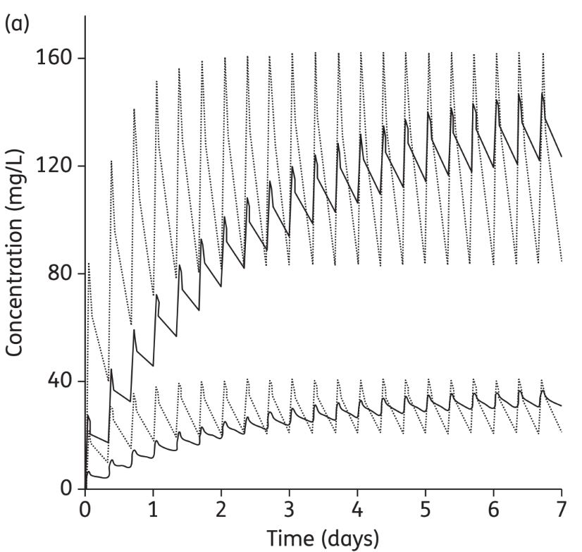
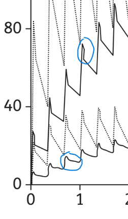
4.3 Figure 2

While it would seem that Figure 2 could also be used for validation of our model implementation, careful consideration of the plot makes us suspect that technical errors happened while preparing the figure. Therefore, no attempt at reproducing the figure will be made.

4.4 Conclusion

We think our mrgsolve model is an adequate representation of the published model since :

  1. The equations and parameters values of our mrgsolve model are identical to the reported ones
  2. Most fT>MIC were accurately reproduced

The slight discrepencies could be due to different simulation settings (e.g. different time points) and/or missing correlations between variability parameters which were not reported.