Article
Rambaud A, Gaborit BJ, Deschanvres C, Le Turnier P, Lecomte R, Asseray-Madani N, Leroy AG, Deslandes G, Dailly É, Jolliet P, Boutoille D, Bellouard R, Gregoire M; Nantes Anti-Microbial Agents PK/PD (NAMAP) study group. Development and validation of a dosing nomogram for amoxicillin in infective endocarditis. J Antimicrob Chemother. 2020 Oct 1;75(10):2941-2950. doi: 10.1093/jac/dkaa232. PMID: 32601687.
Model description
Route of administration: Continuous infusion.
Population size: 107 patients for model development and 53 for validation. There are no significant differences between the characteristics of the two populations.
Free or total concentrations: Total concentrations.
Structural model: 2 compartment model with linear elimination, inter-individual variability (IIV) on all of the parameters
Error model The original residual error model where the standard deviation of each observation modelled by a polynomial equation is weighted by process noise is approximated with a combined proportional and additive error model.
Covariate model: Creatinine clearance (CRCL) estimated using the CKD-EPI formula on the elimination constant (\(K_e\))
\[
K\_{e_i} = TVKe \cdot \left( \frac{CLCR_{i}}{64.92} \right)^{\beta} \cdot e^{\eta*{i}} \
\]with
\(Ke{i}\) : Amoxicillin elimination constant for subject i (\(h^{-1}\))
\(TVKe\) : Typical amoxicillin elimination constant (\(h^{-1}\))
\(\beta\) : Typical effect of CRCL on \(Ke_{i}\)
\(\eta_{i}\) : individual deviation from typical value with normal distribution centered on 0
\(64.92\) : population’s median creatinine clearance (\(mL.min^{-1}\))
Conversion from non-parametric to parametric
The original model is non-parametric. Inter-individual variability given in the form of mean absolute weighted deviation (MAWD) of parameters was converted to log normal inter-individual variability by \[
\sigma \approx MAWD \cdot 1.4826
\] \[
CV = \frac{\sigma}{\theta}
\] \[
\omega^2 = ln(CV^2 + 1)
\]with
\(\sigma\): standard deviation
CV : coefficient of variation
\(\theta\): typical parameter value
\(\omega^2\): variance of \(\eta_{i}\)
Parameters and mrgsolve implementation
Table 1. Model parameter values where \(K_{12}\) is the diffusion rate constant from the central to the peripheral compartment, \(K_{21}\) is the diffusion rate constant from the peripheral to the central compartment, \(K_e\) is the elimination constant, \(V_1\) is the volume of distribution of the central compartment, \(\beta\) is the effect of CRCL on the elimination constant.
| \(V_1\) (L) |
5.70 |
0.0615 |
| \(K_{12}\) (\(h^{-1}\)) |
0.247 |
1.11 |
| \(K_{21}\) (\(h^{-1}\)) |
11.43 |
0.194 |
| \(K_e\) (\(h^{-1}\)) |
1.69 |
0.0367 |
| \(\beta\) |
0.946 |
0.0964 |
A standard value of 0.05 is used for proportional residual error and 1 \(mg.L^{-1}\) for additive residual unexplained variability (RUV).
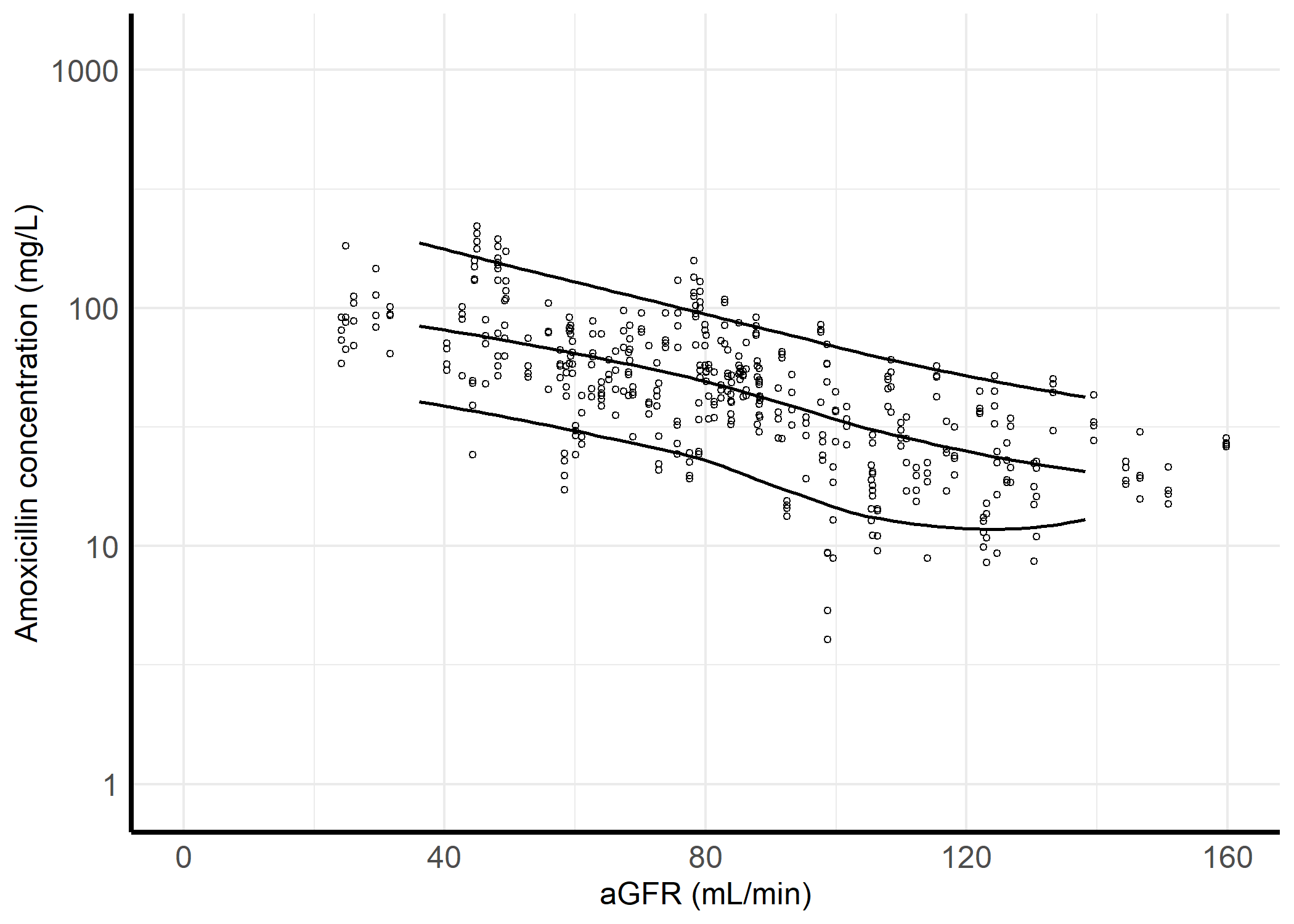
Subject and observation simulation
107 subjects with the characteristics of the model development dataset are simulated. 4 steady-state concentrations are simulated for each subject with the time grid of 72, 96, 120, and 144 h.
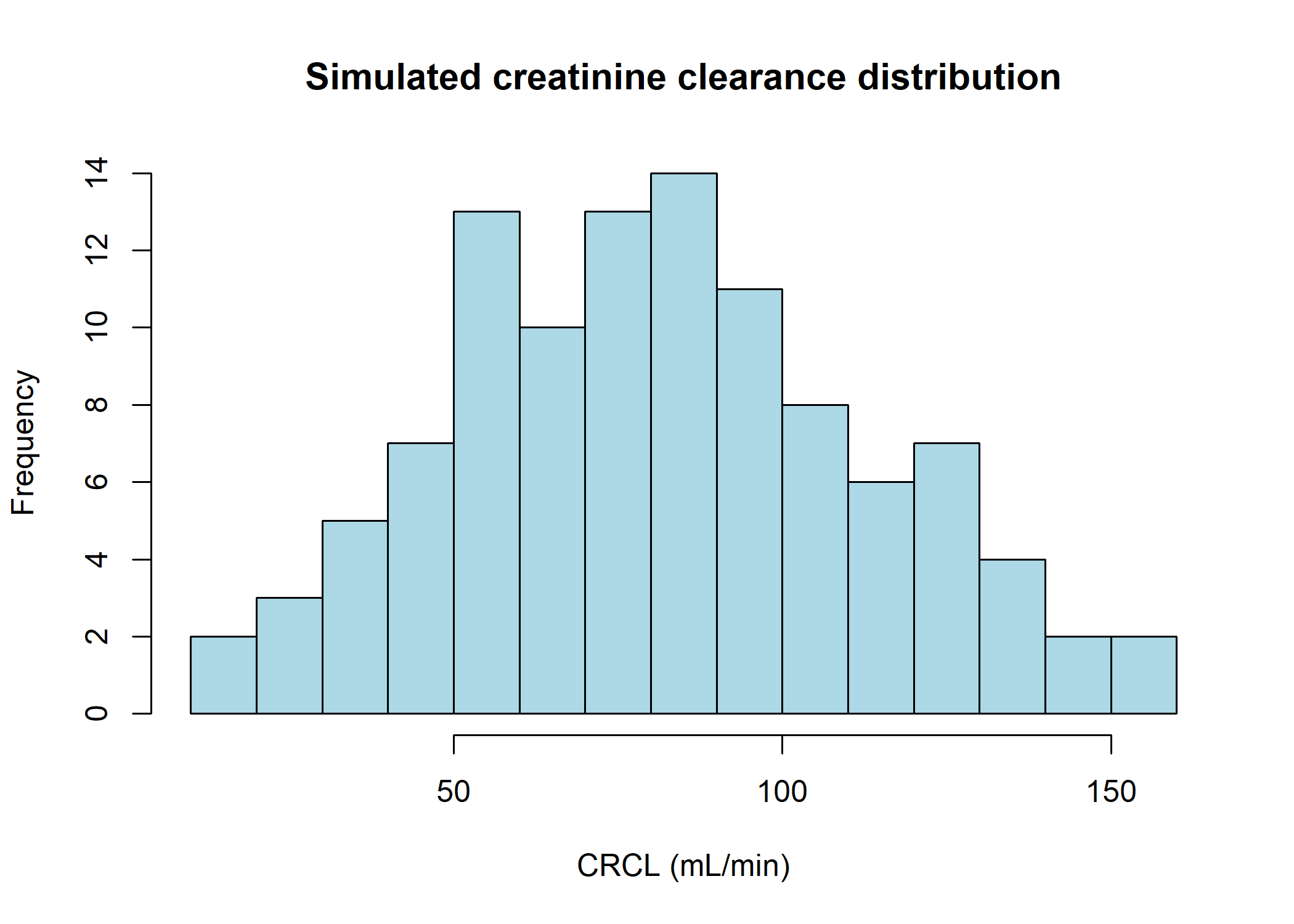
Covariate simulation
Creatinine clearance was simulated with a log-normal distribution using the median (80 \(mL.min^{-1}\)) and interquantile range (52.6 - 106). As the obtained distribution is too narrow compared to the minimum and maximum values read from the figures (\(\approx\) 10 and 160) a small proportion of extra values are simulated in the ranges 10-30 and 140-160. The simulations are iterated until the desired interquantile range is obtained with a maximum difference of 2.
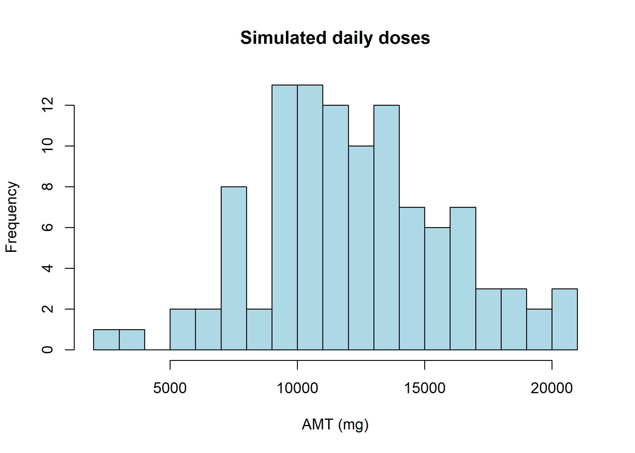
Dose simulation
Doses are simulated with a normal distribution between 2000 mg and 20000 mg with a median of 12000 mg. The doses are rounded to the nearest 500 mg.
The events table is generated with adding the times, CMT and EVID
Checking parameter distributions
Since we relied on approximations to convert the MAWD to log-normal standard deviations, we will check whether the MAWD computed from simulated parameter distributions are close to the ones reported in the paper
| K12 |
0.1524385 |
0.237 |
35.7 % |
| K21 |
3.1753618 |
3.570 |
11.1 % |
| CCRCL |
0.1947902 |
0.203 |
4 % |
| KE1 |
0.2197522 |
0.220 |
0.1 % |
| Vc |
0.9723197 |
0.968 |
-0.4 % |
The relative difference is below 10% for all parameters but K12 (KCP in the paper). This is not of concern because K12 and K21 are not of importance in this specific case.
Indeed when we compute the peripheral volume of this bi-compartmental model we realize that it is negligible when compared with the central compartment volume. \[
Vp = K12/K21 \times Vc = 0.247 / 11.427 \times 5.698 = 0.123 L \]
Thus having a bad representation of transfer to (and from) the peripheral compartment will not cause any problems.
It is worthwhile to note that the data used in the paper only includes concentrations measured after continuous infusions of amoxicillin. In this case, the PK parameters describing peripheral distribution are not identifiable which explains the very low \(Vp\) value.