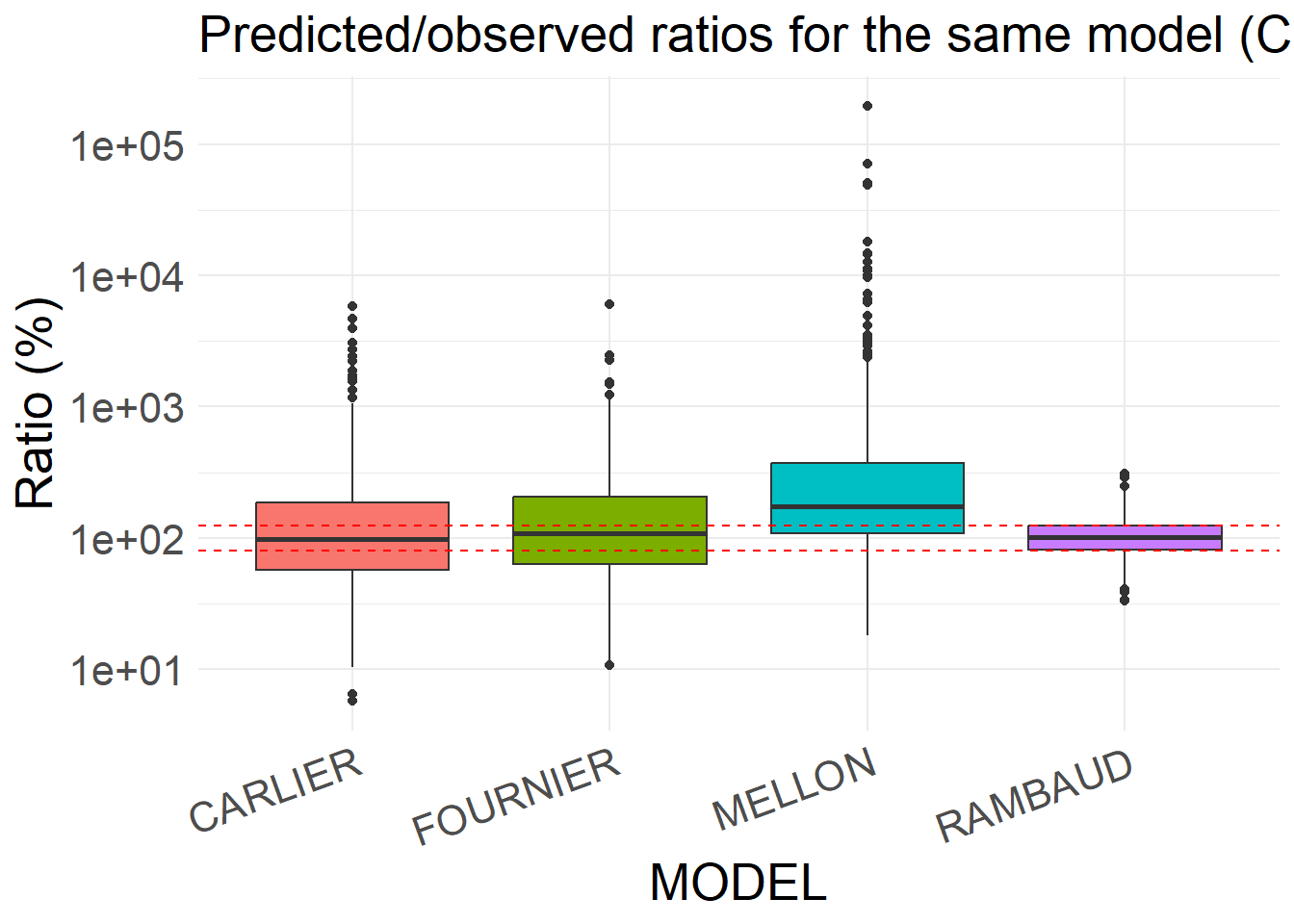
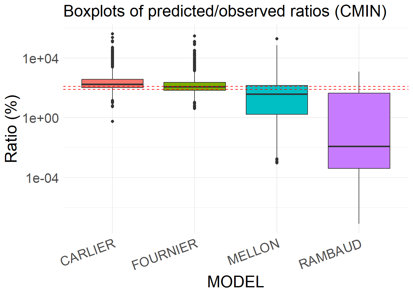
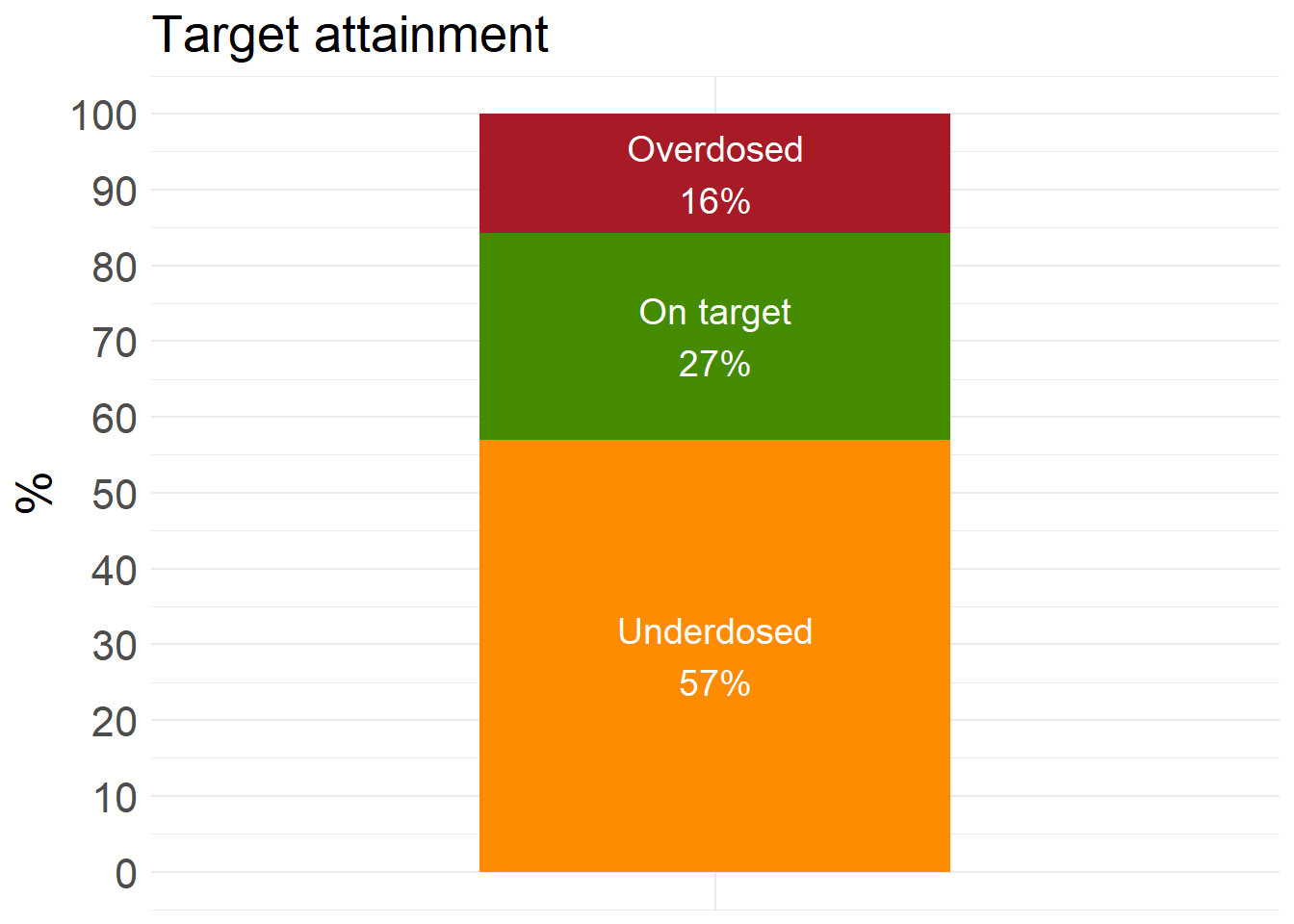
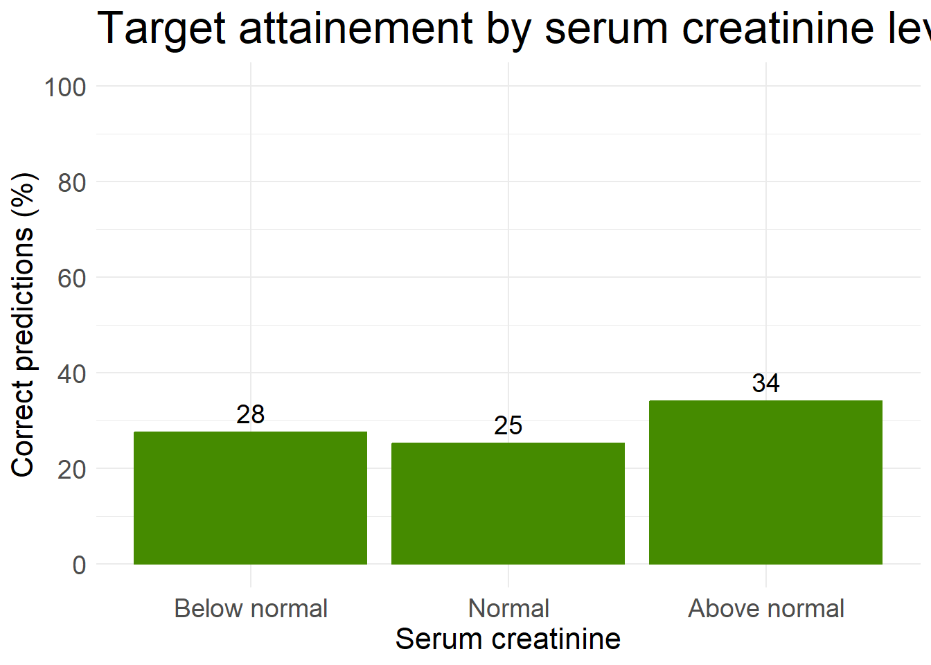
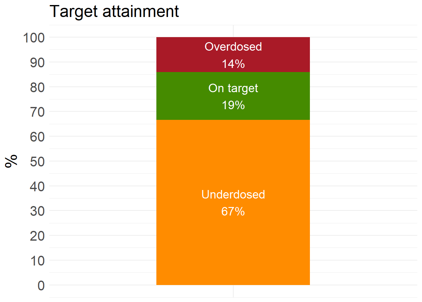
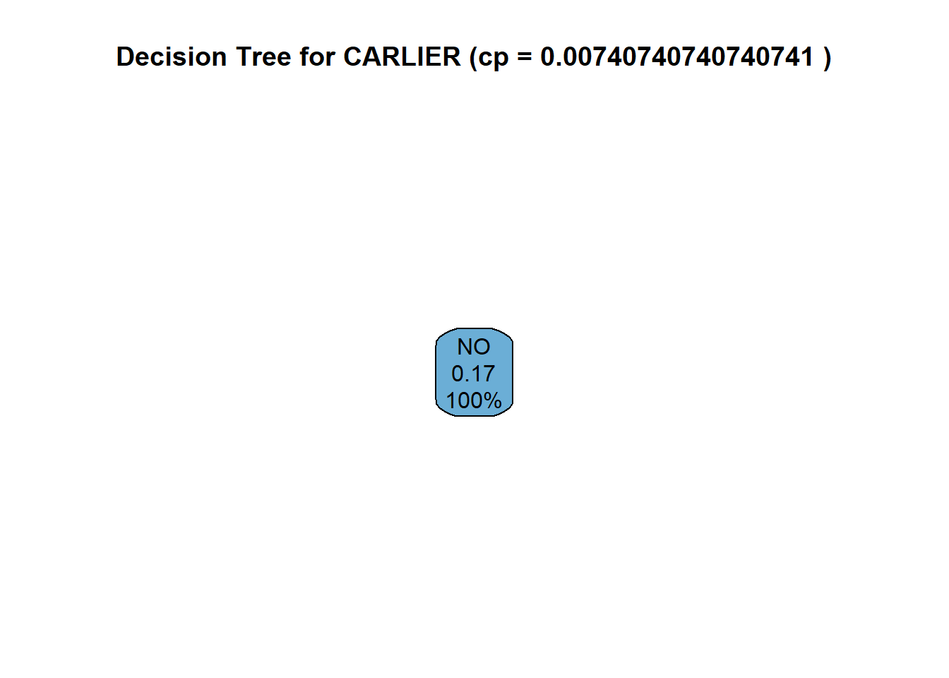
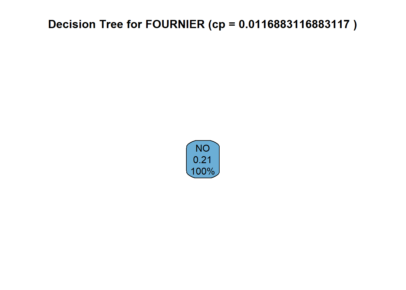
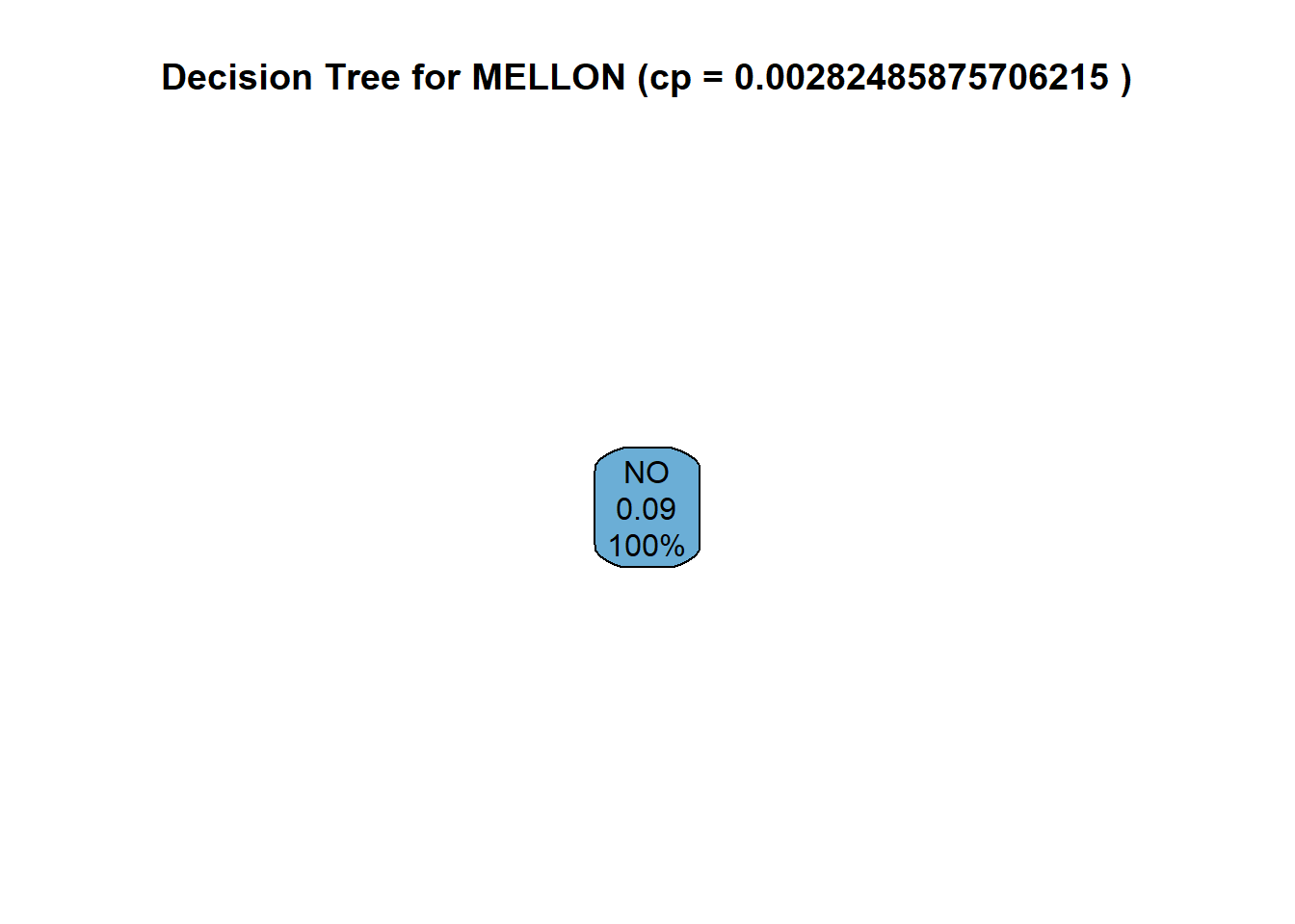
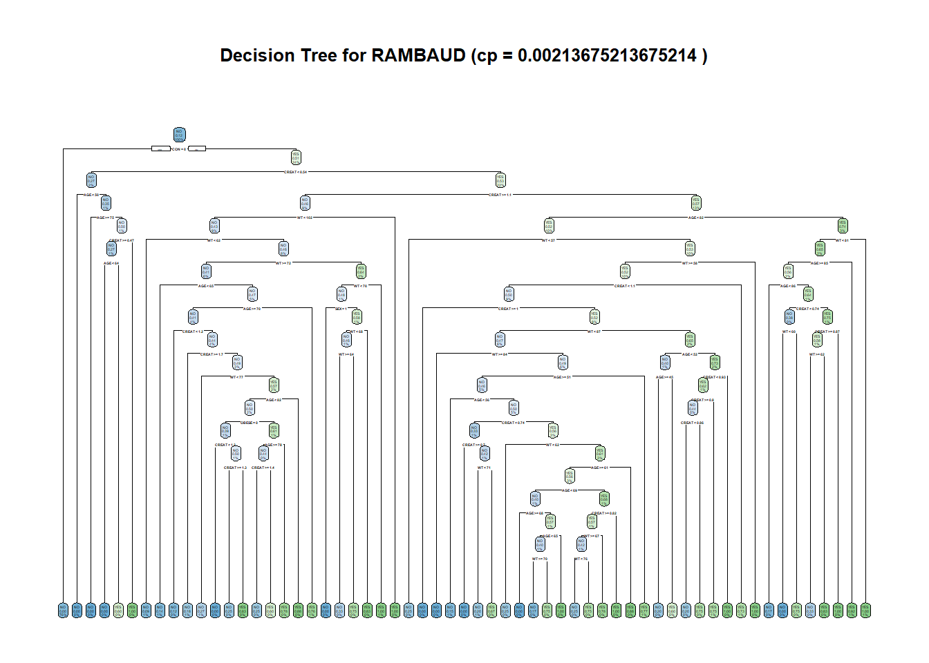
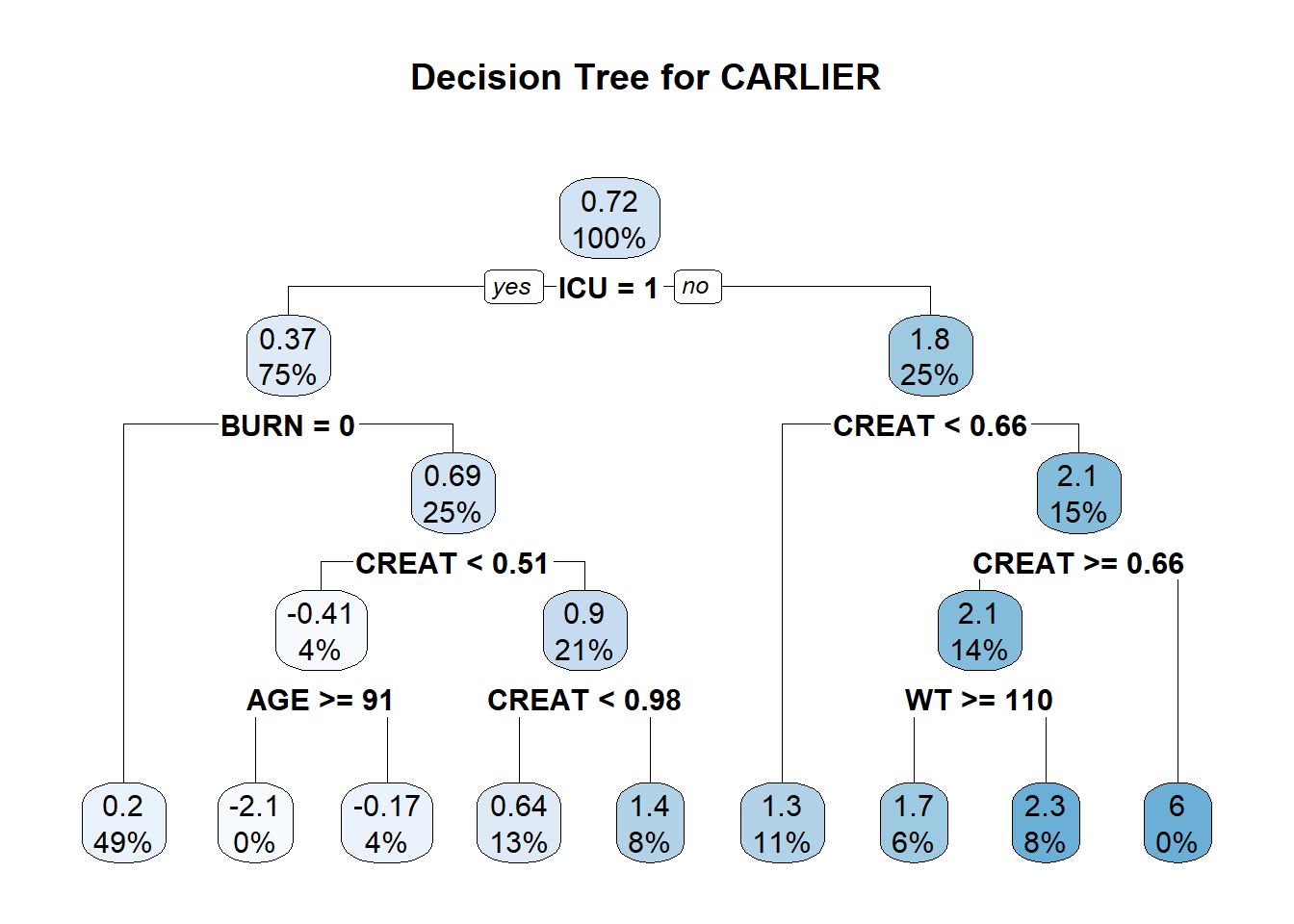
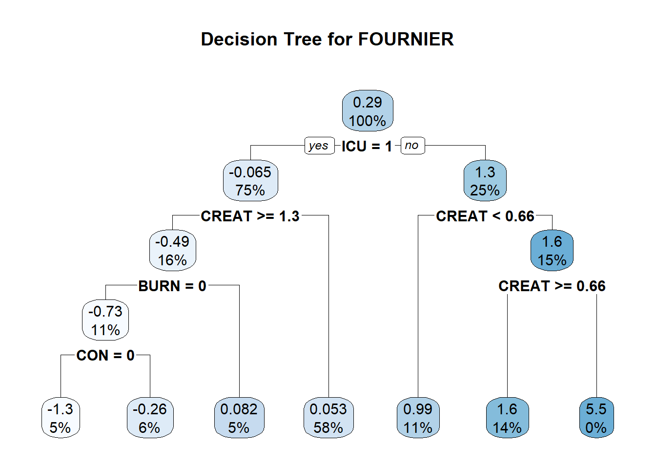
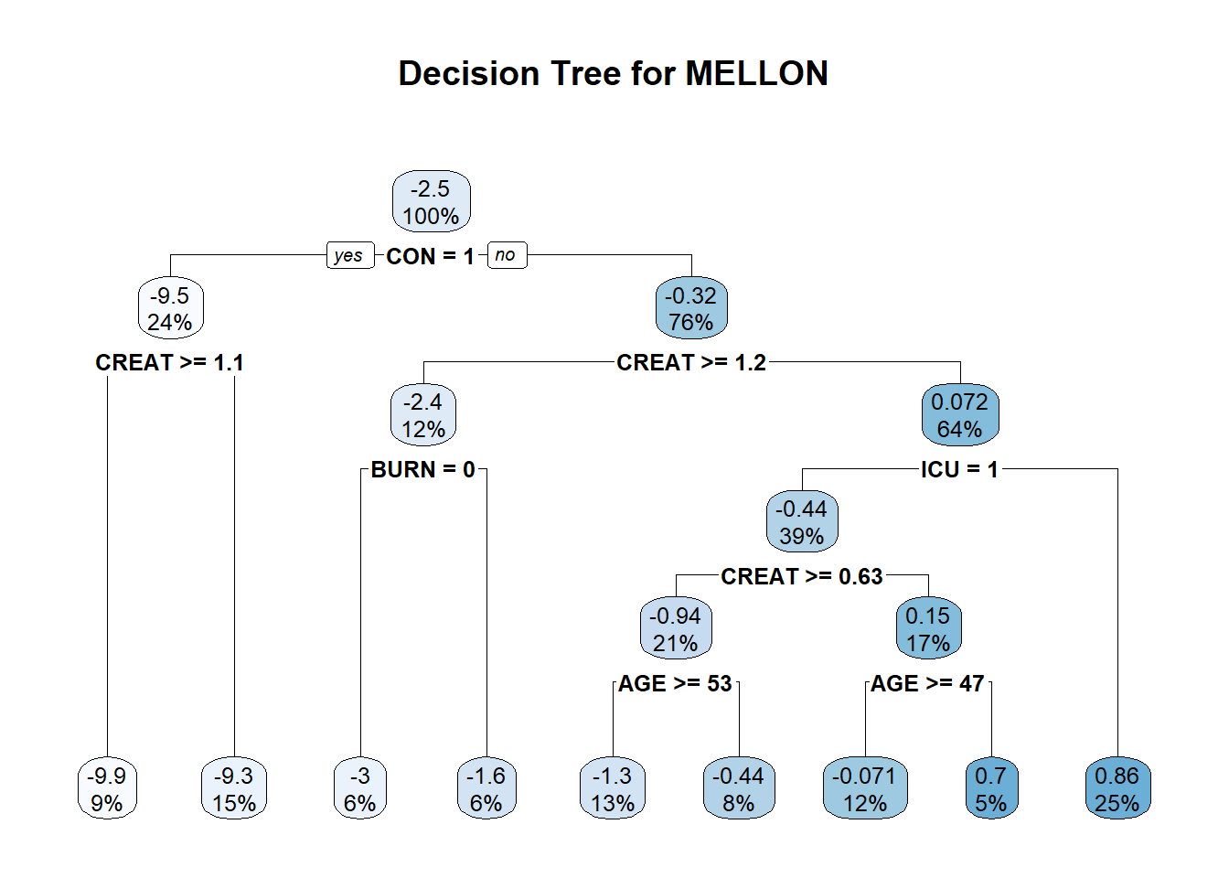
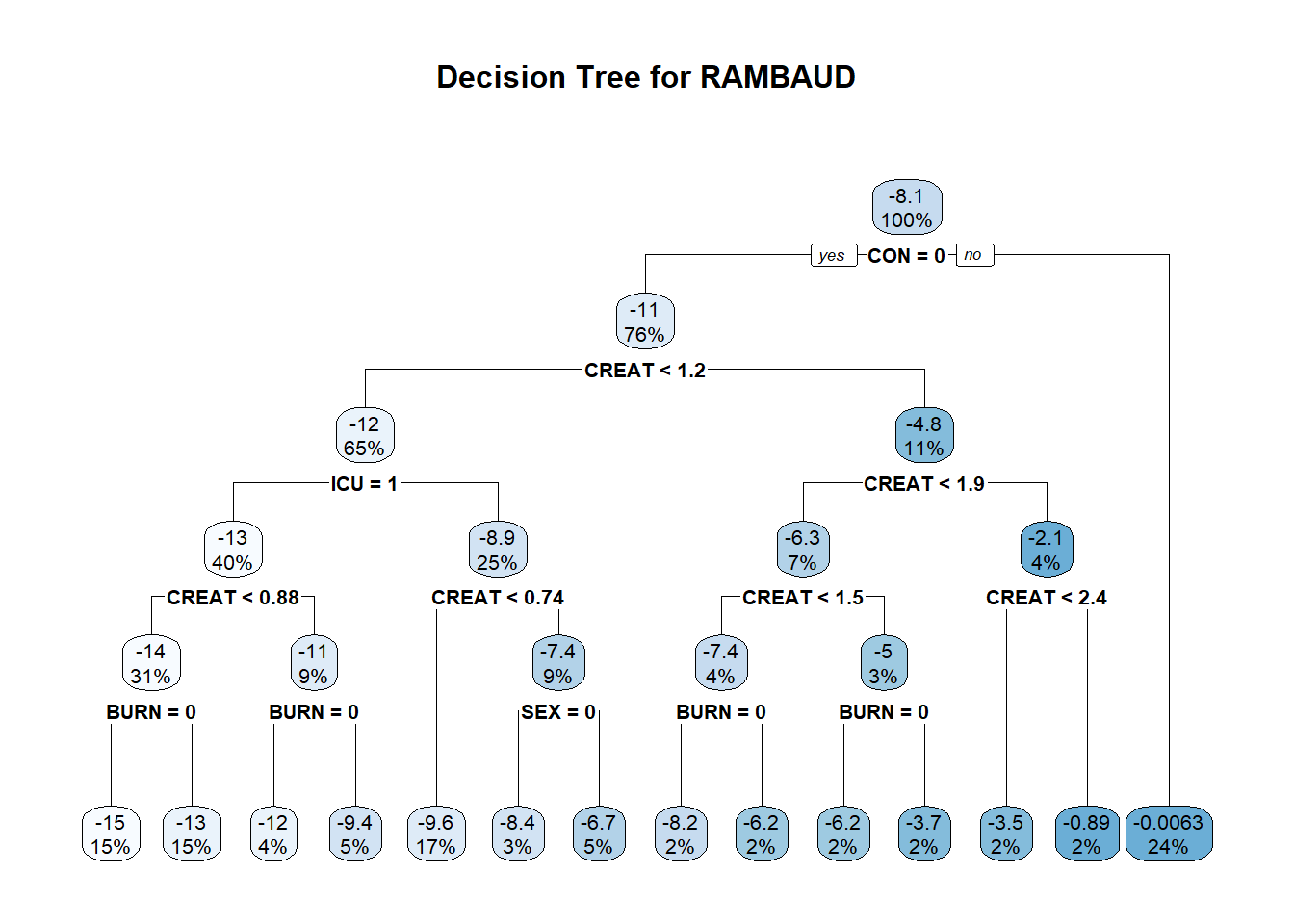
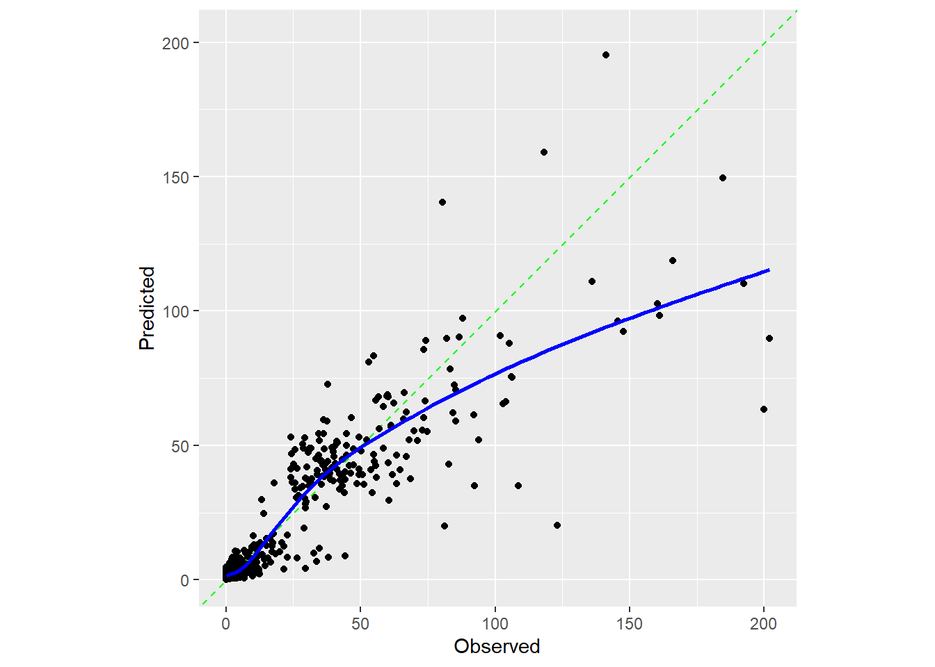
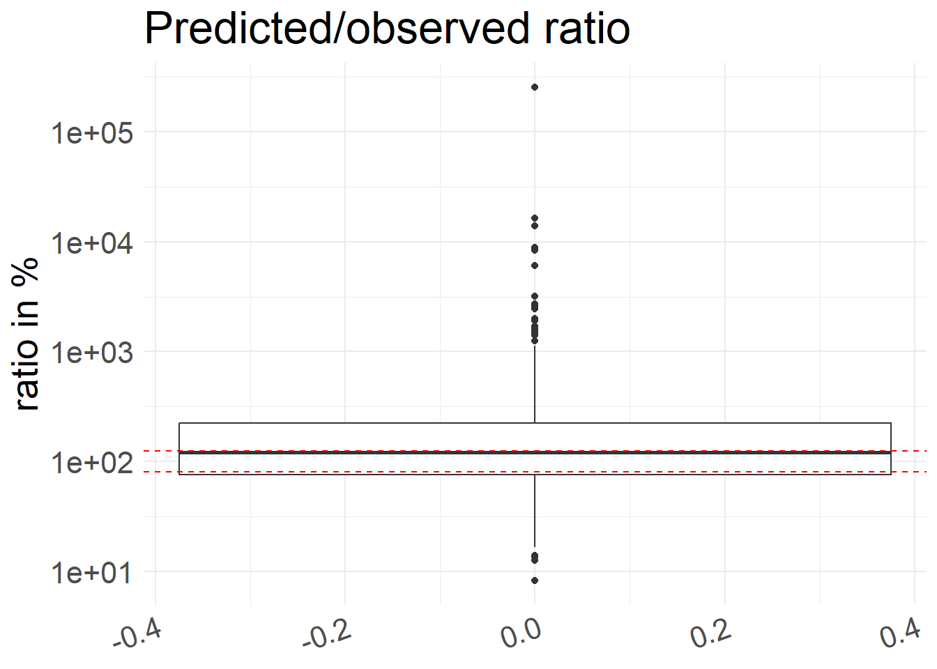
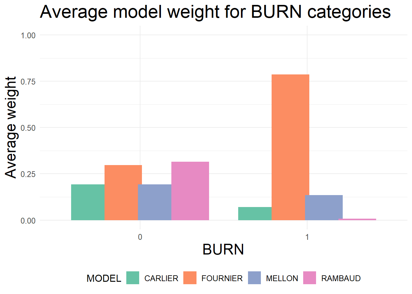
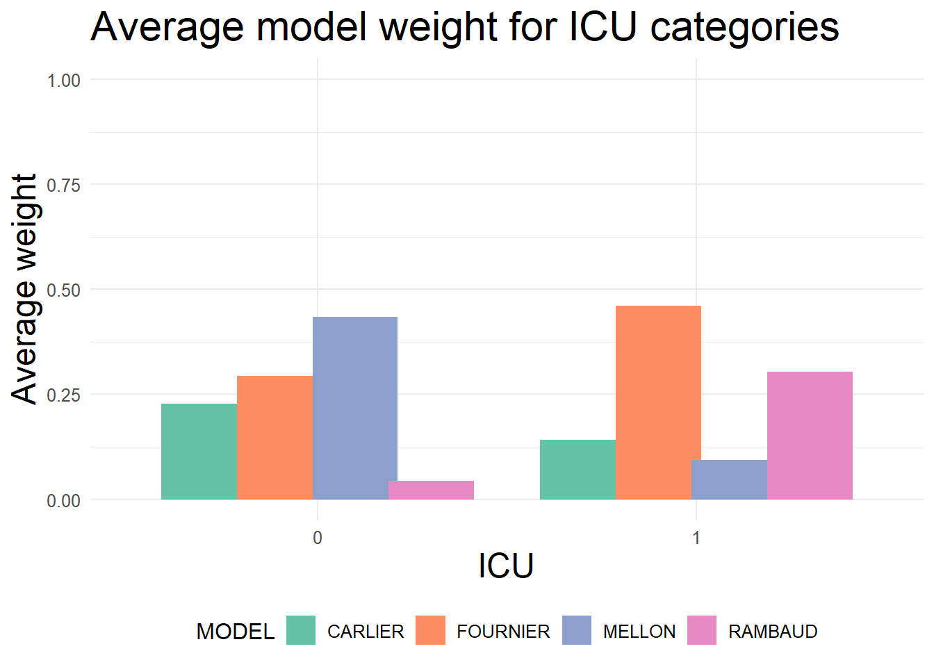
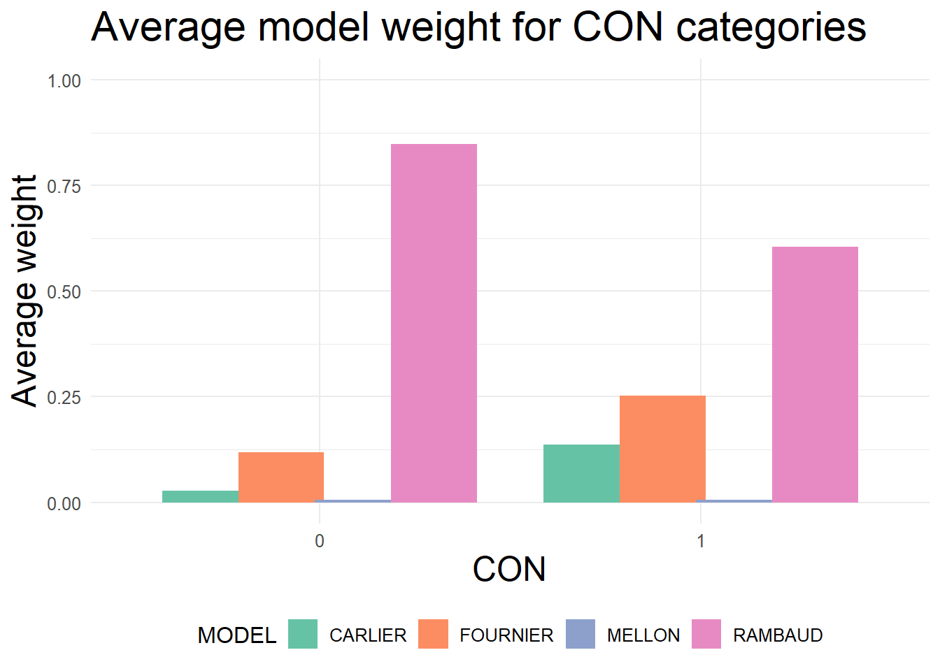
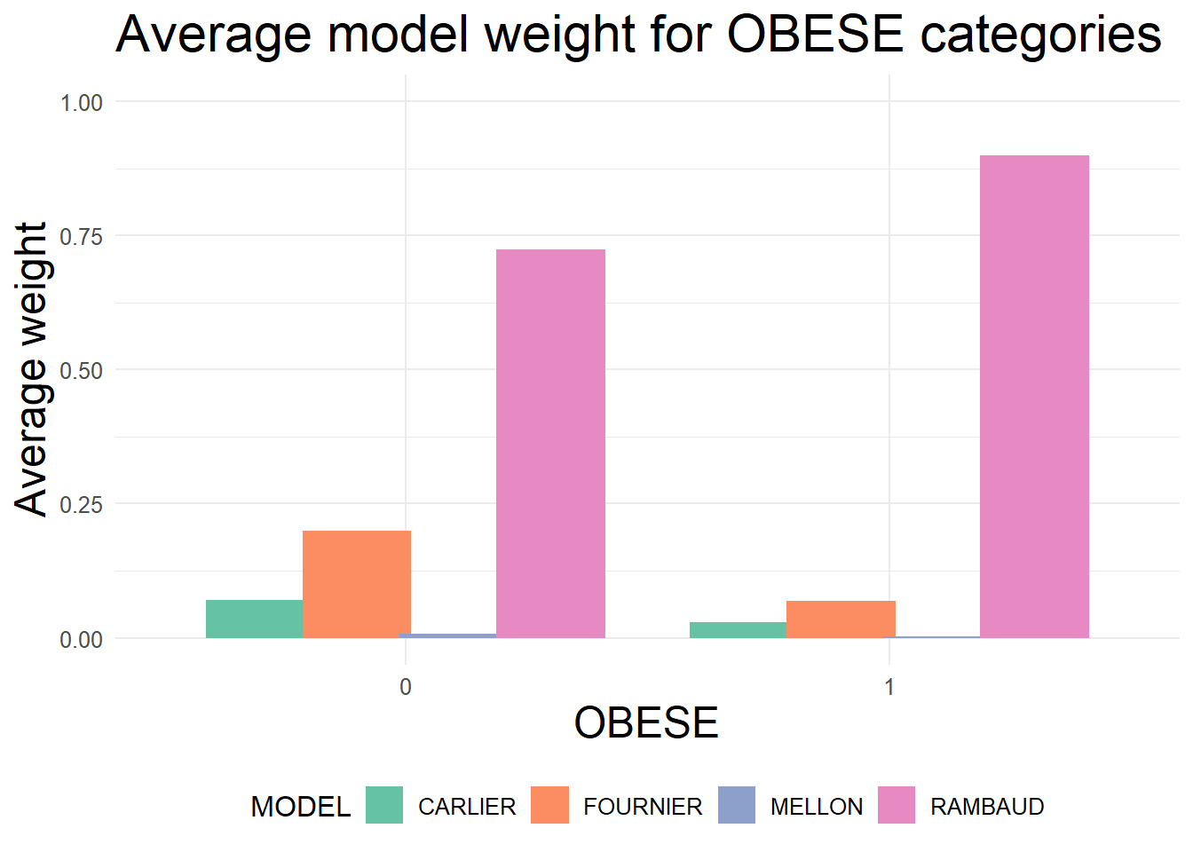
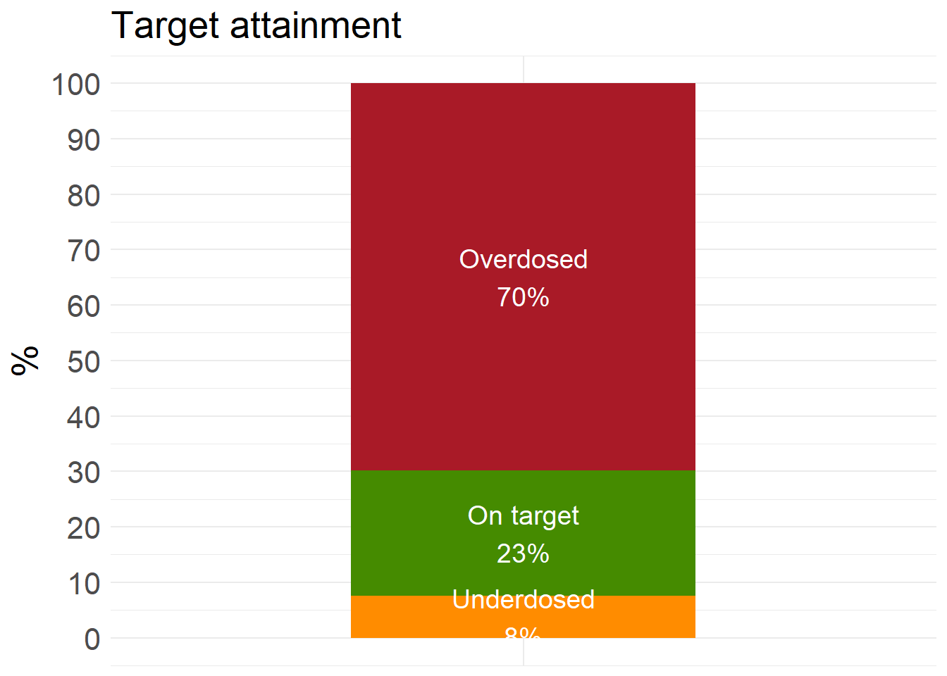
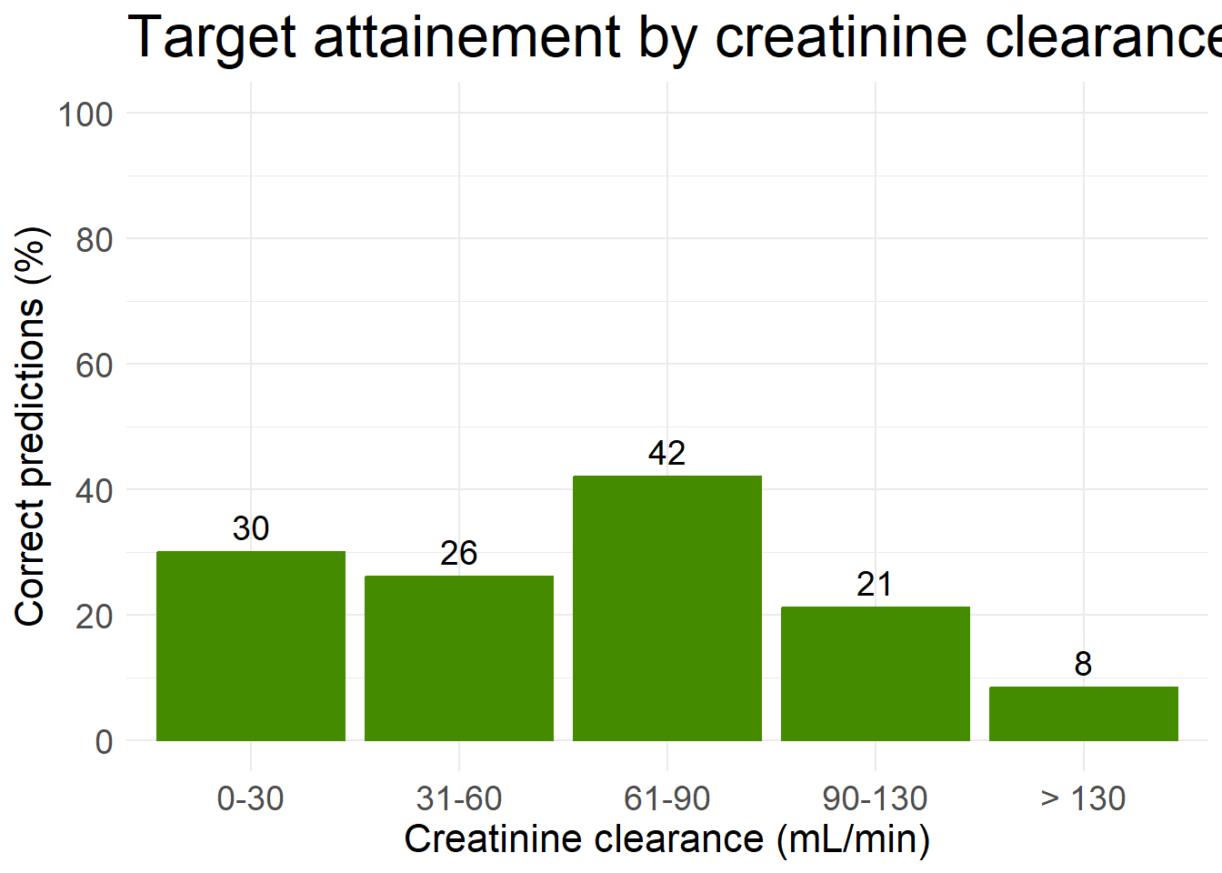
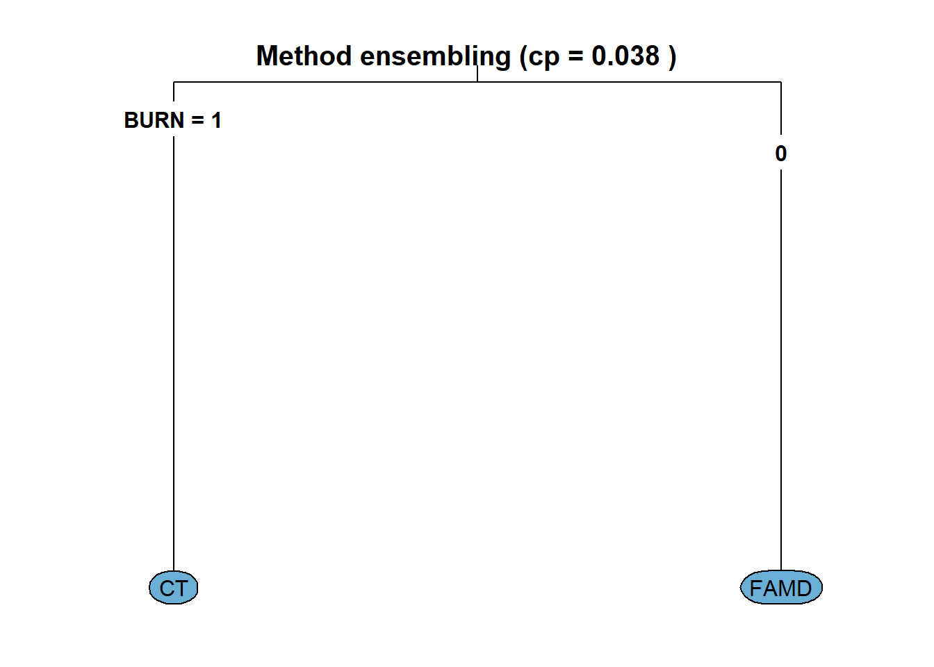
8  Precision dosing approaches

Show the code
library(here)
here::i_am("MIPD/Precision_dosing_methods.qmd")

library(openMIPD)
library(dplyr)
library(ggplot2)
library(readr)
library(tidyr)
library(rpart.plot)
library(ggplot2)
library(patchwork)
library(mrgsolve)
library(kernlab)
library(purrr)

set.seed(1991)

9 Generate predictions with each model

Show the code
AMOX_CMIN_OBS_TRAIN <- read.csv(here("Data/AMOX_CMIN_OBS_TRAIN.csv"), quote = "") |> 
  mutate(
    SEX_CAT = case_when(
      SEX == 0 ~ "M",
      SEX == 1 ~ "F"
    )
  ) |>
  rowwise() |> 
  mutate(CRCL_CKD_EPI_BSA_NORM = estimate_GFR(AGE,CREAT,SEX_CAT)) |> 
  ungroup() |> 
  mutate(CRCL_CKD_EPI_ABSOLUTE = CRCL_CKD_EPI_BSA_NORM * (BSA/1.73))

AMOX_CMIN_OBS_TEST <- read.csv(here("Data/AMOX_CMIN_OBS_TEST.csv"), quote = "") |> 
  mutate(
    SEX_CAT = case_when(
      SEX == 0 ~ "M",
      SEX == 1 ~ "F"
    )
  ) |>
  rowwise() |> 
  mutate(CRCL_CKD_EPI_BSA_NORM = estimate_GFR(AGE,CREAT,SEX_CAT)) |> 
  ungroup() |> 
  mutate(CRCL_CKD_EPI_ABSOLUTE = CRCL_CKD_EPI_BSA_NORM * (BSA/1.73))
Show the code
perform_mrgsolve_prediction <- function(input_data,
                                        mrgsolve_model_path,
                                        model_name,
                                        cmin_target) {
  
  full_data <- select(input_data,-MODEL) #MODEL column identifies the model with which the prediction was made thus we have to drop it to be able to join later on

data_for_mrgsolve <- input_data |>
  select(
    ID,
    TIME,
    CREAT,
    BURN,
    ICU,
    OBESE,
    AGE,
    SEX,
    HT,
    BSA,
    DOSE_ADM,
    FREQ,
    DUR,
    CMIN_IND,
    MODEL_COHORT
  ) |> distinct()

mrgsolve_model <- mread_cache(mrgsolve_model_path)

mrgsolve_dose_data <- 
      rename(data_for_mrgsolve,
           AMT = DOSE_ADM,
           II = FREQ
           ) |> 
  mutate(RATE = AMT/DUR,
         ADDL = TIME/II - 1,
         TIME = 0,
         EVID = 1,
         CMT = 1)

mrgsolve_obs_data <- rename(data_for_mrgsolve,
           AMT = DOSE_ADM,
           II = FREQ
           ) |> 
  mutate(RATE = NA,
         ADDL = NA,
         EVID = 0,
         CMT = 1)
  
mrgsolve_input_data <- bind_rows(mrgsolve_dose_data,
                                        mrgsolve_obs_data) |> 
  arrange(ID,-EVID)

mrgsolve_model |> 
  data_set(mrgsolve_input_data) |> 
  zero_re() |>  
  mrgsim(obsonly = TRUE,
         recover = colnames(mrgsolve_input_data)) |>
  as_tibble() |> 
  rename(CMIN_PRED = IPRED) |> 
  mutate(MODEL = model_name) |> 
  select(ID,MODEL,CMIN_PRED) |> 
  right_join(full_data) |> 
  mutate(DOSE_PRED = cmin_target/CMIN_PRED * DOSE_ADM)
  
}

9.1 CARLIER

Show the code
AMOX_CMIN_PRED_TRAIN_CARLIER <- perform_mrgsolve_prediction(
  input_data = AMOX_CMIN_OBS_TRAIN ,
  mrgsolve_model_path = here(
    "Simulations/amox_Carlier"
  ),
  model_name = "CARLIER",
  cmin_target = 60 #mg/L
) 

AMOX_CMIN_PRED_TEST_CARLIER <- perform_mrgsolve_prediction(
  input_data = AMOX_CMIN_OBS_TEST ,
  mrgsolve_model_path = here(
    "Simulations/amox_Carlier"
  ),
  model_name = "CARLIER",
  cmin_target = 60 #mg/L
) 

9.2 FOURNIER

Show the code
AMOX_CMIN_PRED_TRAIN_FOURNIER <- perform_mrgsolve_prediction(
  input_data = AMOX_CMIN_OBS_TRAIN ,
  mrgsolve_model_path = here(
    "Simulations/amox_Fournier"
  ),
  model_name = "FOURNIER",
  cmin_target = 60 #mg/L
) 

AMOX_CMIN_PRED_TEST_FOURNIER <- perform_mrgsolve_prediction(
  input_data = AMOX_CMIN_OBS_TEST ,
  mrgsolve_model_path = here(
    "Simulations/amox_Fournier"
  ),
  model_name = "FOURNIER",
  cmin_target = 60 #mg/L
) 

9.3 MELLON

Show the code
AMOX_CMIN_PRED_TRAIN_MELLON <- perform_mrgsolve_prediction(
  input_data = AMOX_CMIN_OBS_TRAIN ,
  mrgsolve_model_path = here(
    "Simulations/amox_Mellon"
  ),
  model_name = "MELLON",
  cmin_target = 60 #mg/L
) 

AMOX_CMIN_PRED_TEST_MELLON <- perform_mrgsolve_prediction(
  input_data = AMOX_CMIN_OBS_TEST ,
  mrgsolve_model_path = here(
    "Simulations/amox_Mellon"
  ),
  model_name = "MELLON",
  cmin_target = 60 #mg/L
) 

9.4 RAMBAUD

Show the code
AMOX_CMIN_PRED_TRAIN_RAMBAUD <- perform_mrgsolve_prediction(
  input_data = AMOX_CMIN_OBS_TRAIN ,
  mrgsolve_model_path = here(
    "Simulations/amox_Rambaud"
  ),
  model_name = "RAMBAUD",
  cmin_target = 60 #mg/L
) 

AMOX_CMIN_PRED_TEST_RAMBAUD <- perform_mrgsolve_prediction(
  input_data = AMOX_CMIN_OBS_TEST ,
  mrgsolve_model_path = here(
    "Simulations/amox_Rambaud"
  ),
  model_name = "RAMBAUD",
  cmin_target = 60 #mg/L
) 

9.5 Pool all predictions and save them

Show the code
AMOX_CMIN_TRAIN <- bind_rows(
  AMOX_CMIN_PRED_TRAIN_CARLIER,
  AMOX_CMIN_PRED_TRAIN_FOURNIER,
  AMOX_CMIN_PRED_TRAIN_MELLON,
  AMOX_CMIN_PRED_TRAIN_RAMBAUD
  ) |> 
  arrange(ID,MODEL) |> 
  mutate(REFERENCE = if_else(MODEL == MODEL_COHORT, 1, 0)) # Add a variable called REFERENCE which is 1 for the the line where the model used for simulation is the same as the model cohort (otherwise 0) and take only observed values

write.csv(AMOX_CMIN_TRAIN, here("Data/AMOX_CMIN_TRAIN.csv"), row.names = FALSE, quote = FALSE)

AMOX_CMIN_TEST <- bind_rows(
  AMOX_CMIN_PRED_TEST_CARLIER,
  AMOX_CMIN_PRED_TEST_FOURNIER,
  AMOX_CMIN_PRED_TEST_MELLON,
  AMOX_CMIN_PRED_TEST_RAMBAUD
  ) |> 
  arrange(ID,MODEL) |> 
  mutate(REFERENCE = if_else(MODEL == MODEL_COHORT, 1, 0)) # Add a variable called REFERENCE which is 1 for the the line where the model used for simulation is the same as the model cohort (otherwise 0) and take only observed values

write.csv(AMOX_CMIN_TEST, here("Data/AMOX_CMIN_TEST.csv"), row.names = FALSE, quote = FALSE)

9.6 Global inspection of model predictions

9.6.1 Within-cohort performance (inter-individual variability)

Visualization of the inter-individual variability of models by dividing PRED (predicted) values by IPRED (observed) both generated by the same model.

Show the code
# CMIN
# Divide each PRED by the IPRED reference 
AMOX_CMIN2 <- bind_rows(AMOX_CMIN_TRAIN,AMOX_CMIN_TEST) %>%
  filter(REFERENCE == 1) |> 
  group_by(ID, MODEL) %>%
  mutate(
    ratio = (CMIN_PRED / CMIN_IND) * 100
  ) %>%
  ungroup()

# Boxplot of ratios stratified by model
stratified_ratios_CMIN <- ggplot(AMOX_CMIN2, aes(x = MODEL, y = ratio, fill = MODEL)) +
  geom_boxplot() +
  geom_hline(yintercept = 80, linetype = "dashed", color = "red") + 
  geom_hline(yintercept = 125, linetype = "dashed", color = "red") +
  labs(
    title = "Predicted/observed ratios for the same model (Cmax)",
    x = "MODEL",
    y = "Ratio (%)"
  ) +
  theme_minimal() +
  theme(legend.position = "none") +
  theme(
    axis.text.x = element_text(angle = 20, hjust = 1, size = 16),
    axis.text = element_text(size = 16),    
    axis.title = element_text(size = 20), 
    plot.title = element_text(size=20),
  )

stratified_ratios_CMIN + scale_y_log10()

9.6.2 Full dataset performance (model performance)

In this section, the focus is no longer solely on observed concentrations (IPRED), but the performance of the models is explored by illustrating how the predicted concentrations (PRED) for all the cohorts (not just for covariates on which the model was developed) compare the the observed concentration. Visualization of PRED/IPRED ratios. In all cases we compare PRED (predicted) values to a reference IPRED (observed), which is the IPRED of the model whose cohort was used to simulate a particular set of covariates. Red lines indicate the bioequivalence range of 80-125 %.

Show the code
# CMIN
# Divide each PRED by the IPRED reference 
AMOX_CMIN3 <- bind_rows(AMOX_CMIN_TRAIN,AMOX_CMIN_TEST) %>%
  group_by(ID) %>%
  mutate(
    ref_CMIN = first(CMIN_IND[REFERENCE == 1], default = NA),
    ratio = (CMIN_PRED / ref_CMIN) * 100
  ) %>%
  ungroup()

# Boxplot of ratios stratified by model
perf_CMIN <- ggplot(AMOX_CMIN3, aes(x = MODEL, y = ratio, fill = MODEL)) +
  geom_boxplot() +
  scale_y_log10() +
  geom_hline(yintercept = 80, linetype = "dashed", color = "red") + 
  geom_hline(yintercept = 125, linetype = "dashed", color = "red") +
  labs(
    title = "Boxplots of predicted/observed ratios (CMIN)",
    x = "MODEL",
    y = "Ratio (%)"
  ) +
  theme_minimal() +
  theme(legend.position = "none") +
  theme(
    axis.text.x = element_text(angle = 20, hjust = 1, size = 16),
    axis.text = element_text(size = 16),    
    axis.title = element_text(size = 20), 
    plot.title = element_text(size=20),
  )

perf_CMIN

10 Single model approach

Show the code
explore_predictions <- function(data, conc_inf = 40, conc_sup = 80, freq_column = "FREQ") {
  # Calculate true dose range and prediction correctness
  data <- data %>%
    mutate(
      DOSE_inf = (conc_inf / CMIN_IND) * DOSE_ADM,
      DOSE_sup = (conc_sup / CMIN_IND) * DOSE_ADM
    ) %>%
    mutate(
      Prediction_correctness = ifelse(
        (DOSE_PRED >= DOSE_inf & DOSE_PRED <= DOSE_sup),
        "Correct", "Incorrect"
      )
    ) %>%
    drop_na(Prediction_correctness) %>%
    mutate(
      Dosing = case_when(
        Prediction_correctness == "Correct" ~ "On target",
        DOSE_PRED < DOSE_inf ~ "Underdosed",
        DOSE_PRED > DOSE_sup ~ "Overdosed"
      )
    )

  # Proportions of under- and overdosing
  dosing <- data %>%
    count(Dosing) %>%
    mutate(
      Proportion = n / sum(n) * 100,
      Dosing = factor(Dosing, levels = c("Overdosed", "On target", "Underdosed")),
      Label = paste0(Dosing, "\n", round(Proportion), "%")
    )

  # Over/underdosed graph
  p1 <- ggplot(dosing, aes(x = "", y = Proportion, fill = Dosing)) +
    geom_bar(stat = "identity", width = 0.5) +
    geom_text(aes(label = Label), position = position_stack(vjust = 0.5), color = "white", size = 5) +
    scale_fill_manual(values = c("Underdosed" = "darkorange", "On target" = "chartreuse4", "Overdosed" = "#A91A27")) +
    labs(y = "%", x = NULL, title = "Target attainment", fill = "Dosing Category") +
    theme_minimal() +
    theme(
      axis.text.x = element_blank(),
      axis.ticks.x = element_blank(),
      plot.title = element_text(size = 20),
      axis.text = element_text(size = 16),
      axis.title = element_text(size = 20),
      legend.position = "none"
    ) +
    scale_y_continuous(breaks = seq(0, 100, by = 10)) + 
        coord_cartesian(ylim = c(0, 100))

  # CREAT binning (based on the American Kidney Fund's categories)
data <- data %>%
  mutate(
    CREAT_bin = case_when(# males
      SEX == 0 ~ cut(
        CREAT,
        breaks = c(0, 0.7, 1.3, Inf),
        labels = c("Below normal", "Normal", "Above normal"),
        right = FALSE
      ),
      SEX == 1 ~ cut( # females
        CREAT,
        breaks = c(0, 0.6, 1.1, Inf),
        labels = c("Below normal", "Normal", "Above normal"),
        right = FALSE
      )
    )
  )

  # Binning stats
  bin_summary <- data %>%
    group_by(CREAT_bin, Prediction_correctness) %>%
    summarise(Count = n(), .groups = "drop") %>%
    pivot_wider(names_from = Prediction_correctness, values_from = Count, values_fill = 0) %>%
    mutate(Proportion_Correct = (Correct / (Correct + Incorrect)) * 100)

  # Binning graph
  p2 <- ggplot(bin_summary, aes(x = CREAT_bin, y = Proportion_Correct)) +
    geom_bar(stat = "identity", fill = "chartreuse4", color = "chartreuse4", size = 1) +
    geom_text(aes(label = round(Proportion_Correct)), vjust = -0.5, size = 5, color = "black") +
    labs(title = "Target attainement by serum creatinine level", x = "Serum creatinine", y = "Correct predictions (%)") +
    theme_minimal() +
    theme(
      plot.title = element_text(size = 24),
      axis.text = element_text(size = 14),
      axis.title = element_text(size = 16)
    ) +
    scale_y_continuous(limits = c(0, 100), breaks = seq(0, 100, by = 20))
  
    # CRCL binning for chronic kidney disease categories
data <- data %>%
  mutate(
    CRCL_bin = cut(
        CRCL_CKD_EPI_ABSOLUTE,
        breaks = c(0, 30, 60, 90, 130, Inf),
        labels = c("0-30", "31-60", "61-90",  "90-130",  "> 130"),
        right = FALSE
      )
    )

  # Binning stats
  bin_summary <- data %>%
    group_by(CRCL_bin, Prediction_correctness) %>%
    summarise(Count = n(), .groups = "drop") %>%
    pivot_wider(names_from = Prediction_correctness, values_from = Count, values_fill = 0) %>%
    mutate(Proportion_Correct = (Correct / (Correct + Incorrect)) * 100)

  # Binning graph
  p3 <- ggplot(bin_summary, aes(x = CRCL_bin, y = Proportion_Correct)) +
    geom_bar(stat = "identity", fill = "chartreuse4", color = "chartreuse4", size = 1) +
    geom_text(aes(label = round(Proportion_Correct)), vjust = -0.5, size = 5, color = "black") +
    labs(title = "Target attainement by creatinine clearance category", x = "Creatinine clearance (mL/min)", y = "Correct predictions (%)") +
    theme_minimal() +
    theme(
      plot.title = element_text(size = 24),
      axis.text = element_text(size = 14),
      axis.title = element_text(size = 16)
    ) +
    scale_y_continuous(limits = c(0, 100), breaks = seq(0, 100, by = 20))

  # Summary statistics
  summary_stats <- data %>%
    group_by(Prediction_correctness) %>%
    summarise(
      mean_CREAT = mean(CREAT, na.rm = TRUE),
      sd_CREAT = sd(CREAT, na.rm = TRUE),
      mean_WT = mean(WT, na.rm = TRUE),
      sd_WT = sd(WT, na.rm = TRUE),
      mean_AGE = mean(AGE, na.rm = TRUE),
      sd_AGE = sd(AGE, na.rm = TRUE),
      Count = n()
    ) %>%
    mutate(Proportion = Count / sum(Count))

  correct_proportion <- summary_stats %>%
    filter(Prediction_correctness == "Correct") %>%
    pull(Proportion)

  message(sprintf("Proportion of 'correct' predictions: %.2f%%", correct_proportion * 100))

  return(list(
    target_attainment = p1,
    creat_plot = p2,
    crcl_plot = p3,
    summary_stats = summary_stats
  ))
}

10.1 CARLIER

Show the code
# In this specific case predictions were already
# created before, thus "making predictions"
# simply involve loading them and filtering for the correct model
AMOX_CMIN_PRED_TRAIN_CARLIER <- read_csv(
  here("Data/AMOX_CMIN_TRAIN.csv")
  ) |> 
  filter(MODEL == "CARLIER")

AMOX_CMIN_PRED_TEST_CARLIER <- read_csv(
  here("Data/AMOX_CMIN_TEST.csv")
  ) |> 
  filter(MODEL == "CARLIER")
Show the code
results_carlier_train <- explore_predictions(AMOX_CMIN_PRED_TRAIN_CARLIER)
results_carlier_train$target_attainment 

Show the code
creat_plot_carlier_train <- results_carlier_train$creat_plot
creat_plot_carlier_train

Show the code
crcl_plot_carlier_train <- results_carlier_train$crcl_plot
crcl_plot_carlier_train

Show the code
results_carlier_train$summary_stats 
# A tibble: 2 × 9
  Prediction_correctness mean_CREAT sd_CREAT mean_WT sd_WT mean_AGE sd_AGE Count
  <chr>                       <dbl>    <dbl>   <dbl> <dbl>    <dbl>  <dbl> <int>
1 Correct                     0.982    0.558    79.0  14.2     64.1   17.2   512
2 Incorrect                   0.912    0.606    86.4  19.0     57.4   15.6  1363
# ℹ 1 more variable: Proportion <dbl>
Show the code
results_carlier_test <- explore_predictions(AMOX_CMIN_PRED_TEST_CARLIER)
results_carlier_test$target_attainment 

Show the code
creat_plot_carlier_test <- results_carlier_test$creat_plot
creat_plot_carlier_test

Show the code
crcl_plot_carlier_test <- results_carlier_test$crcl_plot
crcl_plot_carlier_test

Show the code
results_carlier_test$summary_stats 
# A tibble: 2 × 9
  Prediction_correctness mean_CREAT sd_CREAT mean_WT sd_WT mean_AGE sd_AGE Count
  <chr>                       <dbl>    <dbl>   <dbl> <dbl>    <dbl>  <dbl> <int>
1 Correct                     1.02     0.593    79.7  14.8     65.1   17.3   171
2 Incorrect                   0.921    0.571    86.3  19.7     57.9   15.6   429
# ℹ 1 more variable: Proportion <dbl>

10.2 FOURNIER

Show the code
# In this specific case predictions were already
# created before, thus "making predictions"
# simply involve loading them and filtering for the correct model
AMOX_CMIN_PRED_TRAIN_FOURNIER <- read_csv(
  here("Data/AMOX_CMIN_TRAIN.csv")
  ) |> 
  filter(MODEL == "FOURNIER")

AMOX_CMIN_PRED_TEST_FOURNIER <- read_csv(
  here("Data/AMOX_CMIN_TEST.csv")
  ) |> 
  filter(MODEL == "FOURNIER")
Show the code
results_fournier_train <- explore_predictions(AMOX_CMIN_PRED_TRAIN_FOURNIER)
results_fournier_train$target_attainment 

Show the code
creat_plot_fournier_train <- results_fournier_train$creat_plot
creat_plot_fournier_train

Show the code
crcl_plot_fournier_train <- results_fournier_train$crcl_plot
crcl_plot_fournier_train

Show the code
results_fournier_train$summary_stats 
# A tibble: 2 × 9
  Prediction_correctness mean_CREAT sd_CREAT mean_WT sd_WT mean_AGE sd_AGE Count
  <chr>                       <dbl>    <dbl>   <dbl> <dbl>    <dbl>  <dbl> <int>
1 Correct                     0.965    0.608    80.7  16.1     64.1   17.9   605
2 Incorrect                   0.914    0.586    86.1  18.7     56.9   15.0  1270
# ℹ 1 more variable: Proportion <dbl>
Show the code
results_fournier_test <- explore_predictions(AMOX_CMIN_PRED_TEST_FOURNIER)
results_fournier_test$target_attainment 

Show the code
creat_plot_fournier_test <- results_fournier_test$creat_plot
creat_plot_fournier_test

Show the code
crcl_plot_fournier_test <- results_fournier_test$crcl_plot
crcl_plot_fournier_test

Show the code
results_fournier_test$summary_stats 
# A tibble: 2 × 9
  Prediction_correctness mean_CREAT sd_CREAT mean_WT sd_WT mean_AGE sd_AGE Count
  <chr>                       <dbl>    <dbl>   <dbl> <dbl>    <dbl>  <dbl> <int>
1 Correct                     0.907    0.432    79.0  15.8     62.7   16.9   191
2 Incorrect                   0.970    0.635    86.9  19.4     58.6   16.0   409
# ℹ 1 more variable: Proportion <dbl>

10.3 MELLON

Show the code
# In this specific case predictions were already
# created before, thus "making predictions"
# simply involve loading them and filtering for the correct model
AMOX_CMIN_PRED_TRAIN_MELLON <- read_csv(
  here("Data/AMOX_CMIN_TRAIN.csv")
  ) |> 
  filter(MODEL == "MELLON")

AMOX_CMIN_PRED_TEST_MELLON <- read_csv(
  here("Data/AMOX_CMIN_TEST.csv")
  ) |> 
  filter(MODEL == "MELLON")
Show the code
results_mellon_train <- explore_predictions(AMOX_CMIN_PRED_TRAIN_MELLON)
results_mellon_train$target_attainment 

Show the code
creat_plot_mellon_train <- results_mellon_train$creat_plot
creat_plot_mellon_train

Show the code
crcl_plot_mellon_train <- results_mellon_train$crcl_plot
crcl_plot_mellon_train

Show the code
results_mellon_train$summary_stats 
# A tibble: 2 × 9
  Prediction_correctness mean_CREAT sd_CREAT mean_WT sd_WT mean_AGE sd_AGE Count
  <chr>                       <dbl>    <dbl>   <dbl> <dbl>    <dbl>  <dbl> <int>
1 Correct                     0.681    0.177    94.9  19.3     52.9   11.9   290
2 Incorrect                   0.977    0.630    82.4  17.2     60.4   16.8  1585
# ℹ 1 more variable: Proportion <dbl>
Show the code
results_mellon_test <- explore_predictions(AMOX_CMIN_PRED_TEST_MELLON)
results_mellon_test$target_attainment 

Show the code
creat_plot_mellon_test <- results_mellon_test$creat_plot
creat_plot_mellon_test

Show the code
crcl_plot_mellon_test <- results_mellon_test$crcl_plot
crcl_plot_mellon_test

Show the code
results_mellon_test$summary_stats 
# A tibble: 2 × 9
  Prediction_correctness mean_CREAT sd_CREAT mean_WT sd_WT mean_AGE sd_AGE Count
  <chr>                       <dbl>    <dbl>   <dbl> <dbl>    <dbl>  <dbl> <int>
1 Correct                     0.713    0.184    93.0  21.8     49.5   13.1    87
2 Incorrect                   0.990    0.612    82.9  17.7     61.7   16.2   513
# ℹ 1 more variable: Proportion <dbl>

10.4 RAMBAUD

Show the code
# In this specific case predictions were already
# created before, thus "making predictions"
# simply involve loading them and filtering for the correct model
AMOX_CMIN_PRED_TRAIN_RAMBAUD <- read_csv(
  here("Data/AMOX_CMIN_TRAIN.csv")
  ) |> 
  filter(MODEL == "RAMBAUD")

AMOX_CMIN_PRED_TEST_RAMBAUD <- read_csv(
  here("Data/AMOX_CMIN_TEST.csv")
  ) |> 
  filter(MODEL == "RAMBAUD")
Show the code
results_rambaud_train <- explore_predictions(AMOX_CMIN_PRED_TRAIN_RAMBAUD)
results_rambaud_train$target_attainment 

Show the code
creat_plot_rambaud_train <- results_rambaud_train$creat_plot
creat_plot_rambaud_train

Show the code
crcl_plot_rambaud_train <- results_rambaud_train$crcl_plot
crcl_plot_rambaud_train

Show the code
results_rambaud_train$summary_stats 
# A tibble: 2 × 9
  Prediction_correctness mean_CREAT sd_CREAT mean_WT sd_WT mean_AGE sd_AGE Count
  <chr>                       <dbl>    <dbl>   <dbl> <dbl>    <dbl>  <dbl> <int>
1 Correct                     1.07     0.492    77.4  13.6     70.9   14.6   329
2 Incorrect                   0.901    0.609    85.9  18.6     56.7   15.6  1546
# ℹ 1 more variable: Proportion <dbl>
Show the code
results_rambaud_test <- explore_predictions(AMOX_CMIN_PRED_TEST_RAMBAUD)
results_rambaud_test$target_attainment 

Show the code
creat_plot_rambaud_test <- results_rambaud_test$creat_plot
creat_plot_rambaud_test

Show the code
crcl_plot_rambaud_test <- results_rambaud_test$crcl_plot
crcl_plot_rambaud_test

Show the code
results_rambaud_test$summary_stats 
# A tibble: 2 × 9
  Prediction_correctness mean_CREAT sd_CREAT mean_WT sd_WT mean_AGE sd_AGE Count
  <chr>                       <dbl>    <dbl>   <dbl> <dbl>    <dbl>  <dbl> <int>
1 Correct                     1.09     0.645    76.5  15.2     70.1   14.1   104
2 Incorrect                   0.921    0.560    86.1  19.0     57.8   16.0   496
# ℹ 1 more variable: Proportion <dbl>

10.5 Meta model

This is an ensembling method where a PopPK model is built based on data simulated with the four models (Carlier, Fournier, Mellon, and Rambaud).

The model is built on the training set used for the ensembling algorithms and tested on the test set. The data is rich and does not contain below quantification limit concentrations. The 3 three compartment structural model was a better fit than a two compartment one (OFV drop < 0.1 %), however as the estimate of the second peripheral volume was negligeable (< 1 L), the two-compartment model was preferred. The pharmacostatistical model is developed using the automatic statistical model building tool in Monolix 2024R1. The best model has IIV on all parameters with no covariance between them. The error model is combined with log-normal distribution.

The covariate model is built using the automatic SCM tool of Monolix with respective forward and backward p values of 5 and 1 % (Likelihood Ratio Test). CREAT and WT were added on the clearance.

Show the code
AMOX_CMIN_PRED_TEST_META <- perform_mrgsolve_prediction(
  input_data = AMOX_CMIN_OBS_TEST ,
  mrgsolve_model_path = here(
    "MIPD/amox_Meta"
  ),
  model_name = "META",
  cmin_target = 60 #mg/L
) 
Show the code
results_meta_test <- explore_predictions(AMOX_CMIN_PRED_TEST_META)
results_meta_test$target_attainment 

Show the code
creat_plot_meta_test <- results_meta_test$creat_plot
creat_plot_meta_test

Show the code
crcl_plot_meta_test <- results_meta_test$crcl_plot
crcl_plot_meta_test

Show the code
results_meta_test$summary_stats 
# A tibble: 2 × 9
  Prediction_correctness mean_CREAT sd_CREAT mean_WT sd_WT mean_AGE sd_AGE Count
  <chr>                       <dbl>    <dbl>   <dbl> <dbl>    <dbl>  <dbl> <int>
1 Correct                     0.839    0.301    86.3  20.4     60.4   15.7   168
2 Incorrect                   0.993    0.651    83.6  17.9     59.7   16.6   432
# ℹ 1 more variable: Proportion <dbl>

11 Standard dose

Based on the our standard dose screening, out of five potential dosing regimens guided by the SPILF recommendation and hospital practices, 200 mg/kg is selected as standard dose reference as it gave the highest target attainment on clinical data.

Show the code
AMOX_CMIN_PRED_TRAIN_STD <- AMOX_CMIN_TRAIN %>%
  mutate(DOSE_PRED = (200 * WT) / (24/FREQ)) %>%
  dplyr::select(ID, CREAT, WT, BURN, SEX, AGE, HT, FREQ, DOSE_ADM, DOSE_PRED, CMIN_IND, SEX, BSA, CRCL_CKD_EPI_ABSOLUTE) %>%
  distinct()

AMOX_CMIN_PRED_TEST_STD <- AMOX_CMIN_TEST %>%
  mutate(DOSE_PRED = (200 * WT) / (24/FREQ)) %>%
  dplyr::select(ID, CREAT, WT, BURN, SEX, AGE, HT, FREQ, DOSE_ADM, DOSE_PRED, CMIN_IND, SEX, BSA, CRCL_CKD_EPI_ABSOLUTE) %>%
  distinct()
Show the code
results_standard_train <- explore_predictions(AMOX_CMIN_PRED_TRAIN_STD)
results_standard_train$target_attainment 

Show the code
results_standard_train$creat_plot

Show the code
results_standard_train$summary_stats 
# A tibble: 2 × 9
  Prediction_correctness mean_CREAT sd_CREAT mean_WT sd_WT mean_AGE sd_AGE Count
  <chr>                       <dbl>    <dbl>   <dbl> <dbl>    <dbl>  <dbl> <int>
1 Correct                     1.19     0.743    76.9  12.0     70.1   14.5   291
2 Incorrect                   0.883    0.549    85.7  18.7     57.2   15.8  1584
# ℹ 1 more variable: Proportion <dbl>
Show the code
results_standard_test <- explore_predictions(AMOX_CMIN_PRED_TEST_STD)
results_standard_test$target_attainment 

Show the code
results_standard_test$creat_plot

Show the code
results_standard_test$summary_stats 
# A tibble: 2 × 9
  Prediction_correctness mean_CREAT sd_CREAT mean_WT sd_WT mean_AGE sd_AGE Count
  <chr>                       <dbl>    <dbl>   <dbl> <dbl>    <dbl>  <dbl> <int>
1 Correct                     1.10     0.511    77.7  13.2     70.4   13.7    93
2 Incorrect                   0.923    0.587    85.6  19.3     58.0   16.1   507
# ℹ 1 more variable: Proportion <dbl>

12 Uninformed model ensembling

All the models are given the same weight (one quarter in this case). The performance of the models or the development cohort characteristics are not taken into account.

Show the code
AMOX_CMIN_PRED_TRAIN_UNINF_MOD_ENS <-  AMOX_CMIN_TRAIN %>%
  mutate(WEIGHT = 0.25) %>% # Add uniform weight
  mutate(WEIGHTED_PRED = CMIN_PRED * WEIGHT) %>% # Weigh prediction
  group_by(ID) %>%
  mutate(WEIGHTED_PREDICTION = sum(WEIGHTED_PRED)) %>% # Ensemble weighted predictions
  ungroup() %>%
  dplyr::select(ID, CREAT, WT, BURN, SEX, AGE, HT, FREQ, DOSE_ADM, WEIGHTED_PREDICTION, CMIN_IND, SEX, CRCL_CKD_EPI_ABSOLUTE) %>%
  distinct() %>%
  dplyr::mutate(DOSE_PRED = (60/WEIGHTED_PREDICTION) * DOSE_ADM) # Administered dose extrapolation to reach 60 mg/L

AMOX_CMIN_PRED_TEST_UNINF_MOD_ENS <- AMOX_CMIN_TEST %>%
  mutate(WEIGHT = 0.25) %>% # Add uniform weight
  mutate(WEIGHTED_PRED = CMIN_PRED * WEIGHT) %>% # Weigh prediction
  group_by(ID) %>%
  mutate(WEIGHTED_PREDICTION = sum(WEIGHTED_PRED)) %>% # Ensemble weighted predictions
  ungroup() %>%
  dplyr::select(ID, CREAT, WT, BURN, SEX, AGE, HT, FREQ, DOSE_ADM, WEIGHTED_PREDICTION, CMIN_IND, SEX, CRCL_CKD_EPI_ABSOLUTE) %>%
  distinct() %>%
  dplyr::mutate(DOSE_PRED = (60/WEIGHTED_PREDICTION) * DOSE_ADM) # Administered dose extrapolation to reach 60 mg/L
Show the code
results_uninf_mod_ens_train <- explore_predictions(AMOX_CMIN_PRED_TRAIN_UNINF_MOD_ENS)
results_uninf_mod_ens_train$target_attainment 

Show the code
results_uninf_mod_ens_train$creat_plot

Show the code
results_uninf_mod_ens_train$summary_stats 
# A tibble: 2 × 9
  Prediction_correctness mean_CREAT sd_CREAT mean_WT sd_WT mean_AGE sd_AGE Count
  <chr>                       <dbl>    <dbl>   <dbl> <dbl>    <dbl>  <dbl> <int>
1 Correct                     0.939    0.468    82.8  17.8     62.0   17.0   613
2 Incorrect                   0.927    0.646    85.1  18.2     57.8   15.8  1262
# ℹ 1 more variable: Proportion <dbl>
Show the code
results_uninf_mod_ens_test <- explore_predictions(AMOX_CMIN_PRED_TEST_UNINF_MOD_ENS)
results_uninf_mod_ens_test$target_attainment 

Show the code
results_uninf_mod_ens_test$creat_plot

Show the code
results_uninf_mod_ens_test$summary_stats 
# A tibble: 2 × 9
  Prediction_correctness mean_CREAT sd_CREAT mean_WT sd_WT mean_AGE sd_AGE Count
  <chr>                       <dbl>    <dbl>   <dbl> <dbl>    <dbl>  <dbl> <int>
1 Correct                     0.937    0.515    82.2  18.6     62.3   16.6   194
2 Incorrect                   0.956    0.607    85.5  18.7     58.8   16.2   406
# ℹ 1 more variable: Proportion <dbl>

13 Nomogram

The nomogram developed by Rambaud et al. (2020) in Nantes which predicts the dose in endocarditis patients based solely on absolute glomerular filtration rate.

The daily dose in g to reach 20 mg/L is predicted by the nomogram based on CRCL in mL/min (x) estimated using the CKD-EPI equation \[ \text{Dose} = 0.0001x^2 + 0.0613x + 1.157 \] and then extrapolated to attain 60 mg/L.

Although the nomogram has been validated only for CRCL between 30 and 120 mL/min and continuous infusion, in this study, it was also evaluated in patients with CRCL outside of this range and applied to intermittent infusion.

Show the code
AMOX_CMIN_PRED_TRAIN_NOMOGRAM <-  AMOX_CMIN_TRAIN %>%
    dplyr::select(ID, CREAT, WT, BURN, SEX, AGE, HT, FREQ, DOSE_ADM, CMIN_IND, SEX, CRCL_CKD_EPI_ABSOLUTE) %>%
  mutate(DOSE_PRED = ((0.0001 * CRCL_CKD_EPI_ABSOLUTE^2 + 0.0613 * CRCL_CKD_EPI_ABSOLUTE + 1.157) * 3000) / (24/FREQ)) |> 
  distinct()

AMOX_CMIN_PRED_TEST_NOMOGRAM <- AMOX_CMIN_TEST %>%
  dplyr::select(ID, CREAT, WT, BURN, SEX, AGE, HT, FREQ, DOSE_ADM, CMIN_IND, SEX, CRCL_CKD_EPI_ABSOLUTE) %>%
  mutate(DOSE_PRED = ((0.0001 * CRCL_CKD_EPI_ABSOLUTE^2 + 0.0613 * CRCL_CKD_EPI_ABSOLUTE + 1.157) * 3000) / (24/FREQ)) |> 
  distinct() 
Show the code
results_nomogram_train <- explore_predictions(AMOX_CMIN_PRED_TRAIN_NOMOGRAM)
results_nomogram_train$target_attainment 

Show the code
results_nomogram_train$creat_plot

Show the code
results_nomogram_train$summary_stats 
# A tibble: 2 × 9
  Prediction_correctness mean_CREAT sd_CREAT mean_WT sd_WT mean_AGE sd_AGE Count
  <chr>                       <dbl>    <dbl>   <dbl> <dbl>    <dbl>  <dbl> <int>
1 Correct                     1.04     0.431    75.6  12.6     67.7   15.7   360
2 Incorrect                   0.905    0.623    86.4  18.6     57.2   15.8  1515
# ℹ 1 more variable: Proportion <dbl>
Show the code
results_nomogram_test <- explore_predictions(AMOX_CMIN_PRED_TEST_NOMOGRAM)
results_nomogram_test$target_attainment 

Show the code
results_nomogram_test$creat_plot

Show the code
results_nomogram_test$summary_stats 
# A tibble: 2 × 9
  Prediction_correctness mean_CREAT sd_CREAT mean_WT sd_WT mean_AGE sd_AGE Count
  <chr>                       <dbl>    <dbl>   <dbl> <dbl>    <dbl>  <dbl> <int>
1 Correct                     1.12     0.587    77.0  13.6     69.8   15.1   129
2 Incorrect                   0.904    0.568    86.4  19.4     57.2   15.7   471
# ℹ 1 more variable: Proportion <dbl>

14 Classification tree informed ensembling

This method is used to attribute weights to models based on their probability to give correct predictions for a set of covariates.

The method is based on Agema et al. (2024).

Bioequivalence ratios between \(Cmin_{\text{pred}}\) and \(Cmin_{\text{ind}}\) are calculated and transformed to a binary variable based on if the ratio is in the bioequivalence range [0.80-1.25] or not. This categorical variable is called CORRECT.

First, for each set of covariates, the ratios between the predicted values of the 4 models are compared to the true value. Then, we add the variable CORRECT which takes the value of YES if the ratio is in the bioequivalence range, and the value of NO, if not.

Then, decision tree is developed where the predictors are the seven covariates and a binary variable indicating continuous or intermittent infusion (CON), and the target variable is the categorical variable named CORRECT. A decision tree is fitted separately for each MODEL where the following parameters need to be defined

- Complexity – a penalty that the information gain has to overcome to add a split. A higher complexity value leads to a smaller tree meaning that subjects are divided into smaller number of categories, so their scores will be less diverse. Comlexity is found by automatic hyperparameter tuning based on cross-validation error.
Minsplit – minimum number of samples to split a node (smaller value, deeper tree).
Minbucket – minimum number of samples in the terminal node (smaller value, deeper tree). Minsplit and minbucket in the range of 2-30 range does not affect the results , so 4 is fixed as a value to have deeper trees.
- xval – number of cross validations. 10-fold cross validation is used (the same number as for the ML methods).
- splitting criterion - entropy or Gini impurity. Gini meausures the frequency (f) with which an element is misclassified:

\[ Gini\ impurity = 2 \cdot f \cdot \left(1 - f \right) \ \] Entropy (called information in rpart) measures the disorder of the predictors as a function of the target:

\[ Entropy = f \cdot log_2(f) \]

Normally, the two splitting criteria give similar results. Entropy is more computationally complex as it uses logarithms.

For certain models, the root node is not split any further (same model score for all subjects).
In the obtained leaf_results table, only the leaf nodes are included with the following columns

  • node - node number

  • var - splitting variable (it always says leaf, as only leaves are included in the table)

  • n- number of subjects per node

  • wt - subject weight (all the subject have the same weight)

  • dev - Gini index

  • yval - the predicted class

  • ncompete - Alternative splitting variables that were not selected for a node but give slightly worse performance than the selected variable. As only leaves are included, there are no competing splitting variables.

  • nsurrogate - Used for missing values. Not applicable to leaves.

  • yval2[, 2] - number of NO for the CORRECT variable

  • yval2[, 3] - number of YES

  • yval2[, 4] - proportion of NO

  • yval2[, 5] - proportion of YES

  • prob_yes - same as yval2[, 5], this column is used later to attribute model weights

  • n_obs - number of observations

To this table, in the path column is added containing all the decisions that led to that particular leaf. Then, this string is transformed to lower and upper limits for continuous and categories for categorical covariates. If there are no upper or lower limits or selected categories, NA is added.

In the original method ( Agema et al. (2024)), the leaves are selected with at least a YES proportion of 0.5 and then the selected models are taken into account with equal weight. Here, all models are used with their respective YES proportions. This way, no subject will end up without a model, and the weights will be more nuancedly calculated. Then, for each subject, the four corresponding nodes are found based on its covariates (one for each model). The probabilites (proportions) of having YES (=prob_yes or score) are normalized by their sum for each subject, so that the scores of the models for a subject will always add up to 1. These normalized scores (=weights) are used to ensemble the model predictions.

Finally, the method is tested by ensembling the predictions of the test data using the weights calibrated base on the training data. The administered dose is extrapolated by dividing the weighted concentration prediction by the target concentration (= 60 mg/L).

Our openMIPD package is used to apply this method.

Show the code
AMOX_CMIN_TRAINED_CT <- classification_tree_model_ensembling_train(
  data = AMOX_CMIN_TRAIN, 
  target_variable = "CMIN", 
  continuous_cov = c("WT", "CREAT", "AGE"), 
  categorical_cov = c("OBESE", "ICU", "BURN", "SEX", "CON"))

[1] "Confusion matrix for model: CARLIER"

 node number: 1 
   root

[1] "Confusion matrix for model: FOURNIER"

 node number: 1 
   root

[1] "Confusion matrix for model: MELLON"

 node number: 1 
   root

[1] "Confusion matrix for model: RAMBAUD"

 node number: 2 
   root
   CON=0

 node number: 12 
   root
   CON=1
   CREAT< 0.5407
   AGE< 50.43

 node number: 26 
   root
   CON=1
   CREAT< 0.5407
   AGE>=50.43
   AGE>=74.79

 node number: 108 
   root
   CON=1
   CREAT< 0.5407
   AGE>=50.43
   AGE< 74.79
   CREAT>=0.4709
   AGE< 63.61

 node number: 109 
   root
   CON=1
   CREAT< 0.5407
   AGE>=50.43
   AGE< 74.79
   CREAT>=0.4709
   AGE>=63.61

 node number: 55 
   root
   CON=1
   CREAT< 0.5407
   AGE>=50.43
   AGE< 74.79
   CREAT< 0.4709

 node number: 56 
   root
   CON=1
   CREAT>=0.5407
   CREAT>=1.146
   WT< 102
   WT< 62.11

 node number: 228 
   root
   CON=1
   CREAT>=0.5407
   CREAT>=1.146
   WT< 102
   WT>=62.11
   WT>=71.67
   AGE< 64.82

 node number: 916 
   root
   CON=1
   CREAT>=0.5407
   CREAT>=1.146
   WT< 102
   WT>=62.11
   WT>=71.67
   AGE>=64.82
   AGE>=69.52
   CREAT< 1.194

 node number: 1834 
   root
   CON=1
   CREAT>=0.5407
   CREAT>=1.146
   WT< 102
   WT>=62.11
   WT>=71.67
   AGE>=64.82
   AGE>=69.52
   CREAT>=1.194
   CREAT>=1.741

 node number: 3670 
   root
   CON=1
   CREAT>=0.5407
   CREAT>=1.146
   WT< 102
   WT>=62.11
   WT>=71.67
   AGE>=64.82
   AGE>=69.52
   CREAT>=1.194
   CREAT< 1.741
   WT< 76.98

 node number: 29368 
   root
   CON=1
   CREAT>=0.5407
   CREAT>=1.146
   WT< 102
   WT>=62.11
   WT>=71.67
   AGE>=64.82
   AGE>=69.52
   CREAT>=1.194
   CREAT< 1.741
   WT>=76.98
   AGE< 81.84
   OBESE=0
   CREAT< 1.239

 node number: 58738 
   root
   CON=1
   CREAT>=0.5407
   CREAT>=1.146
   WT< 102
   WT>=62.11
   WT>=71.67
   AGE>=64.82
   AGE>=69.52
   CREAT>=1.194
   CREAT< 1.741
   WT>=76.98
   AGE< 81.84
   OBESE=0
   CREAT>=1.239
   CREAT>=1.298

 node number: 58739 
   root
   CON=1
   CREAT>=0.5407
   CREAT>=1.146
   WT< 102
   WT>=62.11
   WT>=71.67
   AGE>=64.82
   AGE>=69.52
   CREAT>=1.194
   CREAT< 1.741
   WT>=76.98
   AGE< 81.84
   OBESE=0
   CREAT>=1.239
   CREAT< 1.298

 node number: 58740 
   root
   CON=1
   CREAT>=0.5407
   CREAT>=1.146
   WT< 102
   WT>=62.11
   WT>=71.67
   AGE>=64.82
   AGE>=69.52
   CREAT>=1.194
   CREAT< 1.741
   WT>=76.98
   AGE< 81.84
   OBESE=1
   AGE>=77.57
   CREAT>=1.355

 node number: 58741 
   root
   CON=1
   CREAT>=0.5407
   CREAT>=1.146
   WT< 102
   WT>=62.11
   WT>=71.67
   AGE>=64.82
   AGE>=69.52
   CREAT>=1.194
   CREAT< 1.741
   WT>=76.98
   AGE< 81.84
   OBESE=1
   AGE>=77.57
   CREAT< 1.355

 node number: 29371 
   root
   CON=1
   CREAT>=0.5407
   CREAT>=1.146
   WT< 102
   WT>=62.11
   WT>=71.67
   AGE>=64.82
   AGE>=69.52
   CREAT>=1.194
   CREAT< 1.741
   WT>=76.98
   AGE< 81.84
   OBESE=1
   AGE< 77.57

 node number: 7343 
   root
   CON=1
   CREAT>=0.5407
   CREAT>=1.146
   WT< 102
   WT>=62.11
   WT>=71.67
   AGE>=64.82
   AGE>=69.52
   CREAT>=1.194
   CREAT< 1.741
   WT>=76.98
   AGE>=81.84

 node number: 459 
   root
   CON=1
   CREAT>=0.5407
   CREAT>=1.146
   WT< 102
   WT>=62.11
   WT>=71.67
   AGE>=64.82
   AGE< 69.52

 node number: 460 
   root
   CON=1
   CREAT>=0.5407
   CREAT>=1.146
   WT< 102
   WT>=62.11
   WT< 71.67
   WT< 69.69
   SEX=1

 node number: 1844 
   root
   CON=1
   CREAT>=0.5407
   CREAT>=1.146
   WT< 102
   WT>=62.11
   WT< 71.67
   WT< 69.69
   SEX=0
   WT< 67.65
   WT>=63.78

 node number: 1845 
   root
   CON=1
   CREAT>=0.5407
   CREAT>=1.146
   WT< 102
   WT>=62.11
   WT< 71.67
   WT< 69.69
   SEX=0
   WT< 67.65
   WT< 63.78

 node number: 923 
   root
   CON=1
   CREAT>=0.5407
   CREAT>=1.146
   WT< 102
   WT>=62.11
   WT< 71.67
   WT< 69.69
   SEX=0
   WT>=67.65

 node number: 231 
   root
   CON=1
   CREAT>=0.5407
   CREAT>=1.146
   WT< 102
   WT>=62.11
   WT< 71.67
   WT>=69.69

 node number: 29 
   root
   CON=1
   CREAT>=0.5407
   CREAT>=1.146
   WT>=102

 node number: 60 
   root
   CON=1
   CREAT>=0.5407
   CREAT< 1.146
   AGE< 81.53
   WT< 56.88

 node number: 488 
   root
   CON=1
   CREAT>=0.5407
   CREAT< 1.146
   AGE< 81.53
   WT>=56.88
   WT>=58.14
   CREAT< 1.055
   CREAT>=1.04

 node number: 1956 
   root
   CON=1
   CREAT>=0.5407
   CREAT< 1.146
   AGE< 81.53
   WT>=56.88
   WT>=58.14
   CREAT< 1.055
   CREAT< 1.04
   WT< 86.58
   WT>=84.27

 node number: 7828 
   root
   CON=1
   CREAT>=0.5407
   CREAT< 1.146
   AGE< 81.53
   WT>=56.88
   WT>=58.14
   CREAT< 1.055
   CREAT< 1.04
   WT< 86.58
   WT< 84.27
   AGE>=51.17
   AGE< 55.7

 node number: 31316 
   root
   CON=1
   CREAT>=0.5407
   CREAT< 1.146
   AGE< 81.53
   WT>=56.88
   WT>=58.14
   CREAT< 1.055
   CREAT< 1.04
   WT< 86.58
   WT< 84.27
   AGE>=51.17
   AGE>=55.7
   CREAT< 0.7382
   CREAT>=0.7009

 node number: 62634 
   root
   CON=1
   CREAT>=0.5407
   CREAT< 1.146
   AGE< 81.53
   WT>=56.88
   WT>=58.14
   CREAT< 1.055
   CREAT< 1.04
   WT< 86.58
   WT< 84.27
   AGE>=51.17
   AGE>=55.7
   CREAT< 0.7382
   CREAT< 0.7009
   WT< 70.5

 node number: 62635 
   root
   CON=1
   CREAT>=0.5407
   CREAT< 1.146
   AGE< 81.53
   WT>=56.88
   WT>=58.14
   CREAT< 1.055
   CREAT< 1.04
   WT< 86.58
   WT< 84.27
   AGE>=51.17
   AGE>=55.7
   CREAT< 0.7382
   CREAT< 0.7009
   WT>=70.5

 node number: 31318 
   root
   CON=1
   CREAT>=0.5407
   CREAT< 1.146
   AGE< 81.53
   WT>=56.88
   WT>=58.14
   CREAT< 1.055
   CREAT< 1.04
   WT< 86.58
   WT< 84.27
   AGE>=51.17
   AGE>=55.7
   CREAT>=0.7382
   WT< 61.96

 node number: 250552 
   root
   CON=1
   CREAT>=0.5407
   CREAT< 1.146
   AGE< 81.53
   WT>=56.88
   WT>=58.14
   CREAT< 1.055
   CREAT< 1.04
   WT< 86.58
   WT< 84.27
   AGE>=51.17
   AGE>=55.7
   CREAT>=0.7382
   WT>=61.96
   AGE>=60.53
   AGE< 69.15
   AGE>=67.93

 node number: 1002212 
   root
   CON=1
   CREAT>=0.5407
   CREAT< 1.146
   AGE< 81.53
   WT>=56.88
   WT>=58.14
   CREAT< 1.055
   CREAT< 1.04
   WT< 86.58
   WT< 84.27
   AGE>=51.17
   AGE>=55.7
   CREAT>=0.7382
   WT>=61.96
   AGE>=60.53
   AGE< 69.15
   AGE< 67.93
   AGE< 65.49
   WT>=70.42

 node number: 1002213 
   root
   CON=1
   CREAT>=0.5407
   CREAT< 1.146
   AGE< 81.53
   WT>=56.88
   WT>=58.14
   CREAT< 1.055
   CREAT< 1.04
   WT< 86.58
   WT< 84.27
   AGE>=51.17
   AGE>=55.7
   CREAT>=0.7382
   WT>=61.96
   AGE>=60.53
   AGE< 69.15
   AGE< 67.93
   AGE< 65.49
   WT< 70.42

 node number: 501107 
   root
   CON=1
   CREAT>=0.5407
   CREAT< 1.146
   AGE< 81.53
   WT>=56.88
   WT>=58.14
   CREAT< 1.055
   CREAT< 1.04
   WT< 86.58
   WT< 84.27
   AGE>=51.17
   AGE>=55.7
   CREAT>=0.7382
   WT>=61.96
   AGE>=60.53
   AGE< 69.15
   AGE< 67.93
   AGE>=65.49

 node number: 1002216 
   root
   CON=1
   CREAT>=0.5407
   CREAT< 1.146
   AGE< 81.53
   WT>=56.88
   WT>=58.14
   CREAT< 1.055
   CREAT< 1.04
   WT< 86.58
   WT< 84.27
   AGE>=51.17
   AGE>=55.7
   CREAT>=0.7382
   WT>=61.96
   AGE>=60.53
   AGE>=69.15
   CREAT>=0.8211
   WT>=66.9
   WT< 76.18

 node number: 1002217 
   root
   CON=1
   CREAT>=0.5407
   CREAT< 1.146
   AGE< 81.53
   WT>=56.88
   WT>=58.14
   CREAT< 1.055
   CREAT< 1.04
   WT< 86.58
   WT< 84.27
   AGE>=51.17
   AGE>=55.7
   CREAT>=0.7382
   WT>=61.96
   AGE>=60.53
   AGE>=69.15
   CREAT>=0.8211
   WT>=66.9
   WT>=76.18

 node number: 501109 
   root
   CON=1
   CREAT>=0.5407
   CREAT< 1.146
   AGE< 81.53
   WT>=56.88
   WT>=58.14
   CREAT< 1.055
   CREAT< 1.04
   WT< 86.58
   WT< 84.27
   AGE>=51.17
   AGE>=55.7
   CREAT>=0.7382
   WT>=61.96
   AGE>=60.53
   AGE>=69.15
   CREAT>=0.8211
   WT< 66.9

 node number: 250555 
   root
   CON=1
   CREAT>=0.5407
   CREAT< 1.146
   AGE< 81.53
   WT>=56.88
   WT>=58.14
   CREAT< 1.055
   CREAT< 1.04
   WT< 86.58
   WT< 84.27
   AGE>=51.17
   AGE>=55.7
   CREAT>=0.7382
   WT>=61.96
   AGE>=60.53
   AGE>=69.15
   CREAT< 0.8211

 node number: 62639 
   root
   CON=1
   CREAT>=0.5407
   CREAT< 1.146
   AGE< 81.53
   WT>=56.88
   WT>=58.14
   CREAT< 1.055
   CREAT< 1.04
   WT< 86.58
   WT< 84.27
   AGE>=51.17
   AGE>=55.7
   CREAT>=0.7382
   WT>=61.96
   AGE< 60.53

 node number: 3915 
   root
   CON=1
   CREAT>=0.5407
   CREAT< 1.146
   AGE< 81.53
   WT>=56.88
   WT>=58.14
   CREAT< 1.055
   CREAT< 1.04
   WT< 86.58
   WT< 84.27
   AGE< 51.17

 node number: 3916 
   root
   CON=1
   CREAT>=0.5407
   CREAT< 1.146
   AGE< 81.53
   WT>=56.88
   WT>=58.14
   CREAT< 1.055
   CREAT< 1.04
   WT>=86.58
   AGE< 51.92
   AGE>=44.95

 node number: 3917 
   root
   CON=1
   CREAT>=0.5407
   CREAT< 1.146
   AGE< 81.53
   WT>=56.88
   WT>=58.14
   CREAT< 1.055
   CREAT< 1.04
   WT>=86.58
   AGE< 51.92
   AGE< 44.95

 node number: 15672 
   root
   CON=1
   CREAT>=0.5407
   CREAT< 1.146
   AGE< 81.53
   WT>=56.88
   WT>=58.14
   CREAT< 1.055
   CREAT< 1.04
   WT>=86.58
   AGE>=51.92
   CREAT< 0.926
   CREAT>=0.795
   CREAT< 0.8616

 node number: 15673 
   root
   CON=1
   CREAT>=0.5407
   CREAT< 1.146
   AGE< 81.53
   WT>=56.88
   WT>=58.14
   CREAT< 1.055
   CREAT< 1.04
   WT>=86.58
   AGE>=51.92
   CREAT< 0.926
   CREAT>=0.795
   CREAT>=0.8616

 node number: 7837 
   root
   CON=1
   CREAT>=0.5407
   CREAT< 1.146
   AGE< 81.53
   WT>=56.88
   WT>=58.14
   CREAT< 1.055
   CREAT< 1.04
   WT>=86.58
   AGE>=51.92
   CREAT< 0.926
   CREAT< 0.795

 node number: 3919 
   root
   CON=1
   CREAT>=0.5407
   CREAT< 1.146
   AGE< 81.53
   WT>=56.88
   WT>=58.14
   CREAT< 1.055
   CREAT< 1.04
   WT>=86.58
   AGE>=51.92
   CREAT>=0.926

 node number: 245 
   root
   CON=1
   CREAT>=0.5407
   CREAT< 1.146
   AGE< 81.53
   WT>=56.88
   WT>=58.14
   CREAT>=1.055

 node number: 123 
   root
   CON=1
   CREAT>=0.5407
   CREAT< 1.146
   AGE< 81.53
   WT>=56.88
   WT< 58.14

 node number: 248 
   root
   CON=1
   CREAT>=0.5407
   CREAT< 1.146
   AGE>=81.53
   WT< 80.57
   AGE>=84.67
   AGE< 86.04

 node number: 996 
   root
   CON=1
   CREAT>=0.5407
   CREAT< 1.146
   AGE>=81.53
   WT< 80.57
   AGE>=84.67
   AGE>=86.04
   CREAT< 0.7409
   WT< 60.25

 node number: 997 
   root
   CON=1
   CREAT>=0.5407
   CREAT< 1.146
   AGE>=81.53
   WT< 80.57
   AGE>=84.67
   AGE>=86.04
   CREAT< 0.7409
   WT>=60.25

 node number: 1996 
   root
   CON=1
   CREAT>=0.5407
   CREAT< 1.146
   AGE>=81.53
   WT< 80.57
   AGE>=84.67
   AGE>=86.04
   CREAT>=0.7409
   CREAT>=0.8719
   WT>=61.77

 node number: 1997 
   root
   CON=1
   CREAT>=0.5407
   CREAT< 1.146
   AGE>=81.53
   WT< 80.57
   AGE>=84.67
   AGE>=86.04
   CREAT>=0.7409
   CREAT>=0.8719
   WT< 61.77

 node number: 999 
   root
   CON=1
   CREAT>=0.5407
   CREAT< 1.146
   AGE>=81.53
   WT< 80.57
   AGE>=84.67
   AGE>=86.04
   CREAT>=0.7409
   CREAT< 0.8719

 node number: 125 
   root
   CON=1
   CREAT>=0.5407
   CREAT< 1.146
   AGE>=81.53
   WT< 80.57
   AGE< 84.67

 node number: 63 
   root
   CON=1
   CREAT>=0.5407
   CREAT< 1.146
   AGE>=81.53
   WT>=80.57

To evaluate the method training, the decision trees and their corresponding confusion matrices are visualized. On the visualized nodes, the first line indicates the target variable majority class in that node (YES/NO), the second line the proportion of correct predictions (= proportion of YES), and the third line the percentage of subjects in that particular node.

Show the code
AMOX_CMIN_TRAINED_CT$plot
$obj
n= 1875 

node), split, n, loss, yval, (yprob)
      * denotes terminal node

      1) root 1875 234 NO (0.875200000 0.124800000)  
        2) CON=0 1425   5 NO (0.996491228 0.003508772) *
        3) CON=1 450 221 YES (0.491111111 0.508888889)  
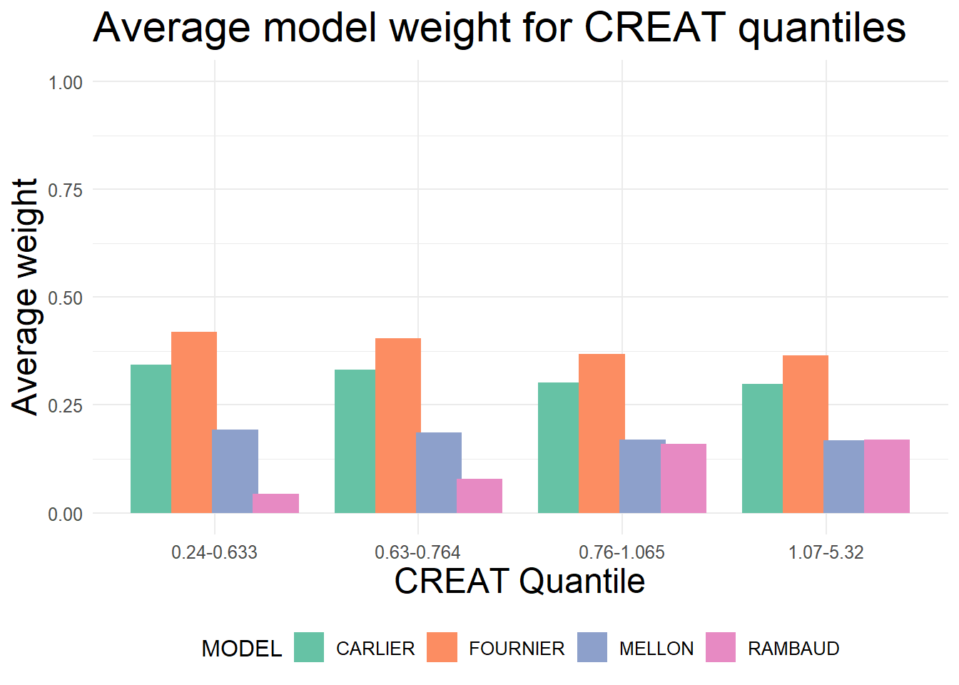
          6) CREAT< 0.5406907 30   8 NO (0.733333333 0.266666667)  
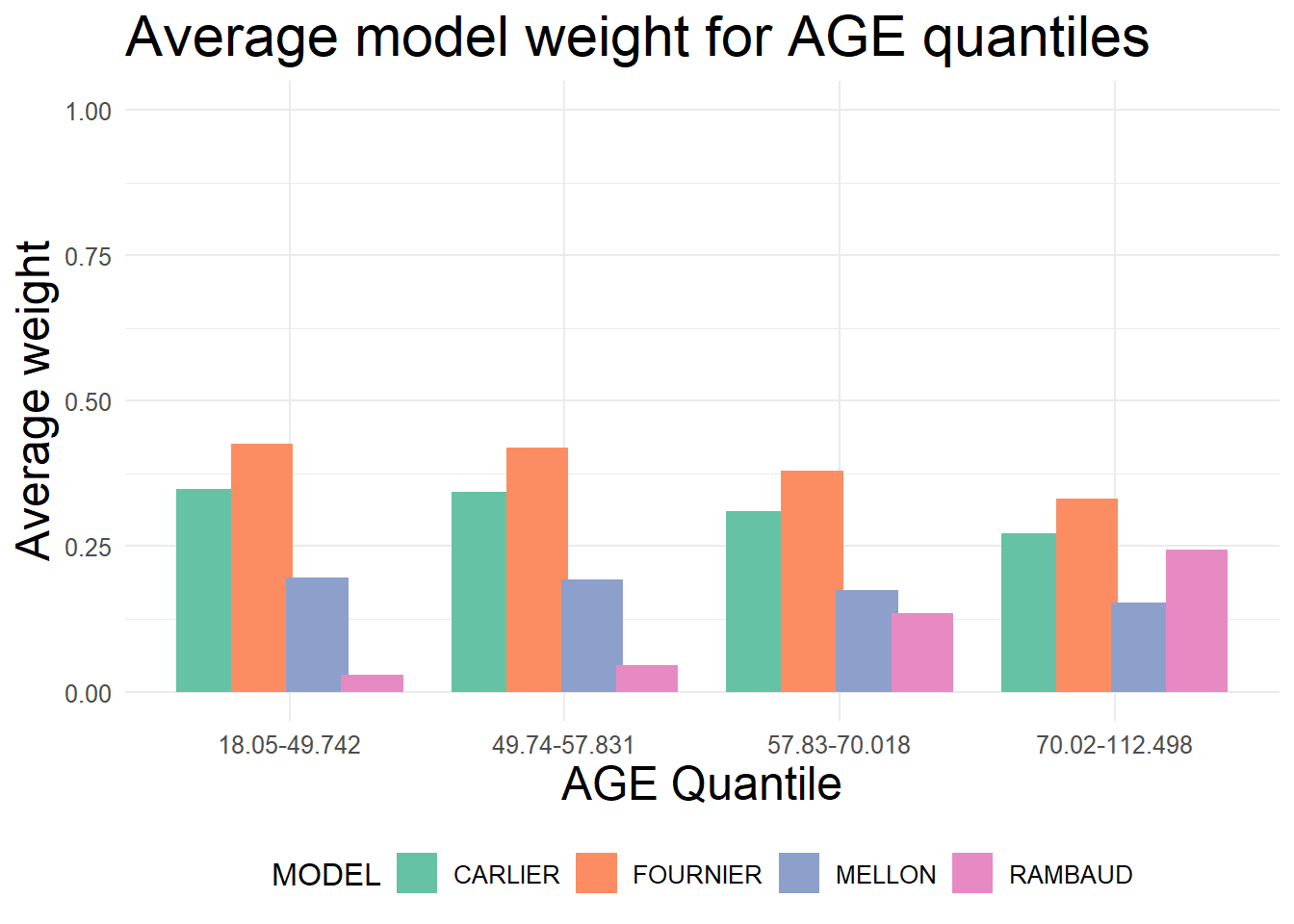
           12) AGE< 50.42605 7   0 NO (1.000000000 0.000000000) *
           13) AGE>=50.42605 23   8 NO (0.652173913 0.347826087)  
             26) AGE>=74.79412 7   0 NO (1.000000000 0.000000000) *
             27) AGE< 74.79412 16   8 NO (0.500000000 0.500000000)  
               54) CREAT>=0.4709054 11   3 NO (0.727272727 0.272727273)  
                108) AGE< 63.61155 6   0 NO (1.000000000 0.000000000) *
                109) AGE>=63.61155 5   2 YES (0.400000000 0.600000000) *
               55) CREAT< 0.4709054 5   0 YES (0.000000000 1.000000000) *
          7) CREAT>=0.5406907 420 199 YES (0.473809524 0.526190476)  
           14) CREAT>=1.146159 167  76 NO (0.544910180 0.455089820)  
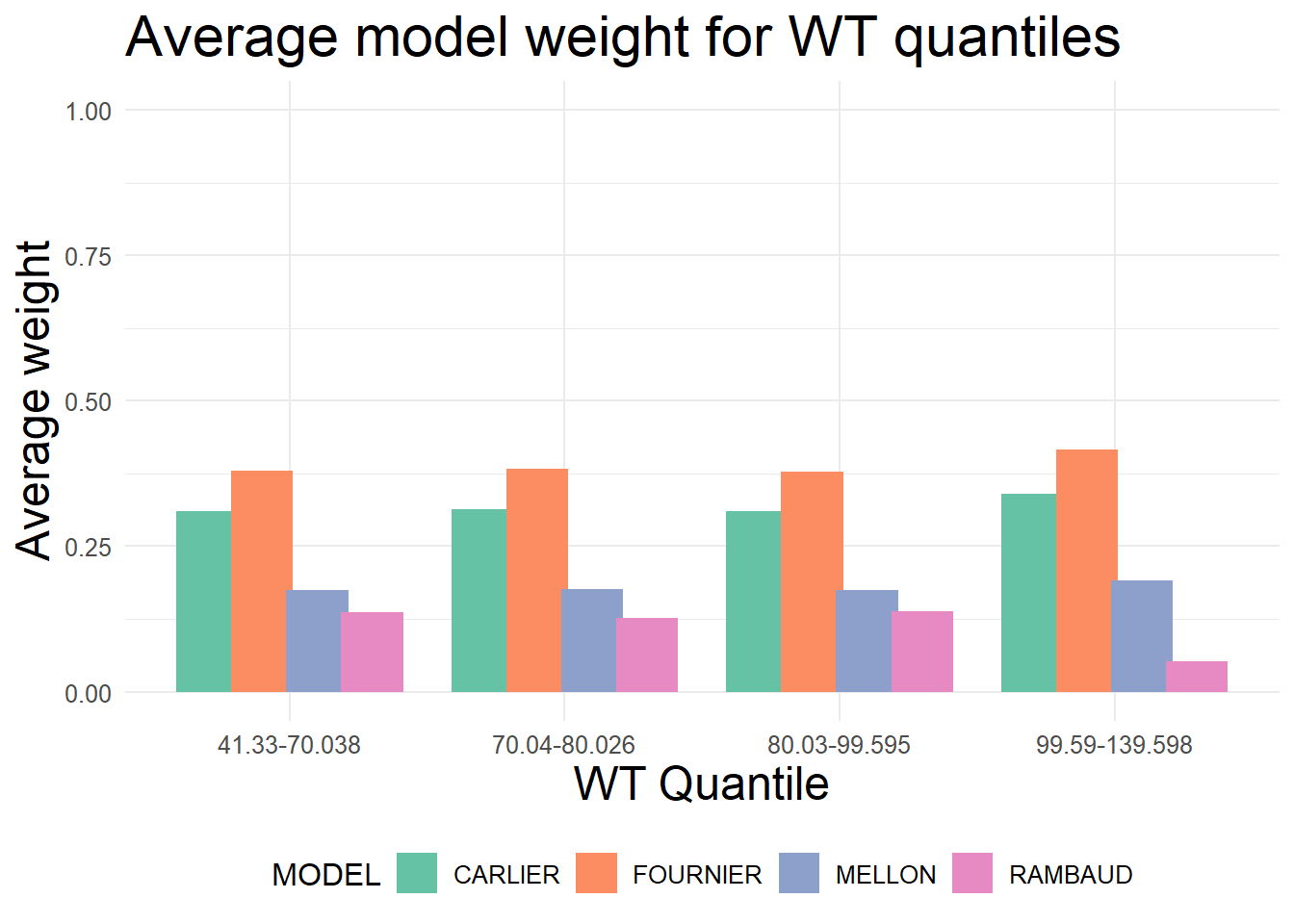
             28) WT< 101.9952 161  70 NO (0.565217391 0.434782609)  
               56) WT< 62.10829 11   1 NO (0.909090909 0.090909091) *
               57) WT>=62.10829 150  69 NO (0.540000000 0.460000000)  
                114) WT>=71.66666 117  48 NO (0.589743590 0.410256410)  
                  228) AGE< 64.82186 22   3 NO (0.863636364 0.136363636) *
                  229) AGE>=64.82186 95  45 NO (0.526315789 0.473684211)  
                    458) AGE>=69.51973 78  32 NO (0.589743590 0.410256410)  
                      916) CREAT< 1.194147 8   1 NO (0.875000000 0.125000000) *
                      917) CREAT>=1.194147 70  31 NO (0.557142857 0.442857143)  
                       1834) CREAT>=1.741118 11   2 NO (0.818181818 0.181818182) *
                       1835) CREAT< 1.741118 59  29 NO (0.508474576 0.491525424)  
                         3670) WT< 76.98115 15   4 NO (0.733333333 0.266666667) *
                         3671) WT>=76.98115 44  19 YES (0.431818182 0.568181818)  
                           7342) AGE< 81.84138 36  18 NO (0.500000000 0.500000000)  
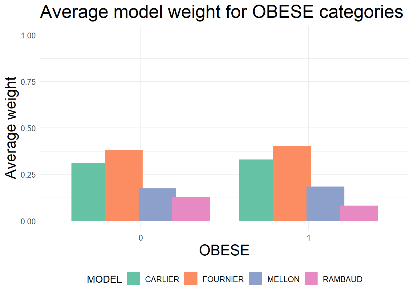
                            14684) OBESE=0 18   7 NO (0.611111111 0.388888889)  
                              29368) CREAT< 1.238723 4   0 NO (1.000000000 0.000000000) *
                              29369) CREAT>=1.238723 14   7 NO (0.500000000 0.500000000)  
                                58738) CREAT>=1.298427 8   2 NO (0.750000000 0.250000000) *
                                58739) CREAT< 1.298427 6   1 YES (0.166666667 0.833333333) *
                            14685) OBESE=1 18   7 YES (0.388888889 0.611111111)  
                              29370) AGE>=77.56952 9   4 NO (0.555555556 0.444444444)  
                                58740) CREAT>=1.354561 4   1 NO (0.750000000 0.250000000) *
                                58741) CREAT< 1.354561 5   2 YES (0.400000000 0.600000000) *
                              29371) AGE< 77.56952 9   2 YES (0.222222222 0.777777778) *
                           7343) AGE>=81.84138 8   1 YES (0.125000000 0.875000000) *
                    459) AGE< 69.51973 17   4 YES (0.235294118 0.764705882) *
                115) WT< 71.66666 33  12 YES (0.363636364 0.636363636)  
                  230) WT< 69.6873 23  11 NO (0.521739130 0.478260870)  
                    460) SEX=1 4   0 NO (1.000000000 0.000000000) *
                    461) SEX=0 19   8 YES (0.421052632 0.578947368)  
                      922) WT< 67.64966 13   6 NO (0.538461538 0.461538462)  
                       1844) WT>=63.77837 9   3 NO (0.666666667 0.333333333) *
                       1845) WT< 63.77837 4   1 YES (0.250000000 0.750000000) *
                      923) WT>=67.64966 6   1 YES (0.166666667 0.833333333) *
                  231) WT>=69.6873 10   0 YES (0.000000000 1.000000000) *
             29) WT>=101.9952 6   0 YES (0.000000000 1.000000000) *
           15) CREAT< 1.146159 253 108 YES (0.426877470 0.573122530)  
             30) AGE< 81.5308 191  92 YES (0.481675393 0.518324607)  
               60) WT< 56.88156 8   2 NO (0.750000000 0.250000000) *
               61) WT>=56.88156 183  86 YES (0.469945355 0.530054645)  
                122) WT>=58.14381 179  86 YES (0.480446927 0.519553073)  
                  244) CREAT< 1.055043 164  82 NO (0.500000000 0.500000000)  
                    488) CREAT>=1.039779 5   0 NO (1.000000000 0.000000000) *
                    489) CREAT< 1.039779 159  77 YES (0.484276730 0.515723270)  
                      978) WT< 86.58055 119  56 NO (0.529411765 0.470588235)  
                       1956) WT>=84.27392 5   0 NO (1.000000000 0.000000000) *
                       1957) WT< 84.27392 114  56 NO (0.508771930 0.491228070)  
                         3914) AGE>=51.17455 101  46 NO (0.544554455 0.455445545)  
                           7828) AGE< 55.70456 13   2 NO (0.846153846 0.153846154) *
                           7829) AGE>=55.70456 88  44 NO (0.500000000 0.500000000)  
                            15658) CREAT< 0.7382098 24   8 NO (0.666666667 0.333333333)  
                              31316) CREAT>=0.7008613 5   0 NO (1.000000000 0.000000000) *
                              31317) CREAT< 0.7008613 19   8 NO (0.578947368 0.421052632)  
                                62634) WT< 70.50466 10   2 NO (0.800000000 0.200000000) *
                                62635) WT>=70.50466 9   3 YES (0.333333333 0.666666667) *
                            15659) CREAT>=0.7382098 64  28 YES (0.437500000 0.562500000)  
                              31318) WT< 61.95855 8   2 NO (0.750000000 0.250000000) *
                              31319) WT>=61.95855 56  22 YES (0.392857143 0.607142857)  
                                62638) AGE>=60.52909 48  21 YES (0.437500000 0.562500000)  
                                 125276) AGE< 69.14929 20   8 NO (0.600000000 0.400000000)  
                                   250552) AGE>=67.92727 6   0 NO (1.000000000 0.000000000) *
                                   250553) AGE< 67.92727 14   6 YES (0.428571429 0.571428571)  
                                     501106) AGE< 65.48585 10   4 NO (0.600000000 0.400000000)  
                                      1002212) WT>=70.41755 6   1 NO (0.833333333 0.166666667) *
                                      1002213) WT< 70.41755 4   1 YES (0.250000000 0.750000000) *
                                     501107) AGE>=65.48585 4   0 YES (0.000000000 1.000000000) *
                                 125277) AGE>=69.14929 28   9 YES (0.321428571 0.678571429)  
                                   250554) CREAT>=0.8210599 21   9 YES (0.428571429 0.571428571)  
                                     501108) WT>=66.90488 12   5 NO (0.583333333 0.416666667)  
                                      1002216) WT< 76.17987 8   2 NO (0.750000000 0.250000000) *
                                      1002217) WT>=76.17987 4   1 YES (0.250000000 0.750000000) *
                                     501109) WT< 66.90488 9   2 YES (0.222222222 0.777777778) *
                                   250555) CREAT< 0.8210599 7   0 YES (0.000000000 1.000000000) *
                                62639) AGE< 60.52909 8   1 YES (0.125000000 0.875000000) *
                         3915) AGE< 51.17455 13   3 YES (0.230769231 0.769230769) *
                      979) WT>=86.58055 40  14 YES (0.350000000 0.650000000)  
                       1958) AGE< 51.91959 10   4 NO (0.600000000 0.400000000)  
                         3916) AGE>=44.95318 5   1 NO (0.800000000 0.200000000) *
                         3917) AGE< 44.95318 5   2 YES (0.400000000 0.600000000) *
                       1959) AGE>=51.91959 30   8 YES (0.266666667 0.733333333)  
                         3918) CREAT< 0.9259867 21   8 YES (0.380952381 0.619047619)  
                           7836) CREAT>=0.7950074 9   4 NO (0.555555556 0.444444444)  
                            15672) CREAT< 0.8615979 5   1 NO (0.800000000 0.200000000) *
                            15673) CREAT>=0.8615979 4   1 YES (0.250000000 0.750000000) *
                           7837) CREAT< 0.7950074 12   3 YES (0.250000000 0.750000000) *
                         3919) CREAT>=0.9259867 9   0 YES (0.000000000 1.000000000) *
                  245) CREAT>=1.055043 15   4 YES (0.266666667 0.733333333) *
                123) WT< 58.14381 4   0 YES (0.000000000 1.000000000) *
             31) AGE>=81.5308 62  16 YES (0.258064516 0.741935484)  
               62) WT< 80.57075 46  16 YES (0.347826087 0.652173913)  
                124) AGE>=84.67447 34  15 YES (0.441176471 0.558823529)  
                  248) AGE< 86.03799 6   1 NO (0.833333333 0.166666667) *
                  249) AGE>=86.03799 28  10 YES (0.357142857 0.642857143)  
                    498) CREAT< 0.7409344 8   3 NO (0.625000000 0.375000000)  
                      996) WT< 60.2531 4   0 NO (1.000000000 0.000000000) *
                      997) WT>=60.2531 4   1 YES (0.250000000 0.750000000) *
                    499) CREAT>=0.7409344 20   5 YES (0.250000000 0.750000000)  
                      998) CREAT>=0.8718551 12   5 YES (0.416666667 0.583333333)  
                       1996) WT>=61.77331 6   2 NO (0.666666667 0.333333333) *
                       1997) WT< 61.77331 6   1 YES (0.166666667 0.833333333) *
                      999) CREAT< 0.8718551 8   0 YES (0.000000000 1.000000000) *
                125) AGE< 84.67447 12   1 YES (0.083333333 0.916666667) *
               63) WT>=80.57075 16   0 YES (0.000000000 1.000000000) *

$snipped.nodes
NULL

$xlim
[1] 0 1

$ylim
[1] 0 1

$x
  [1] 0.148649696 0.004955367 0.292344025 0.040148286 0.022018600 0.058277971
  [7] 0.039081834 0.077474109 0.064676684 0.056145067 0.073208300 0.090271534
 [13] 0.544539764 0.303378654 0.192284341 0.107334767 0.277233914 0.181586493
 [19] 0.124398000 0.238774986 0.165456405 0.141461234 0.189451577 0.158524467
 [25] 0.220378688 0.175587700 0.265169675 0.235309017 0.205448358 0.192650934
 [31] 0.218245783 0.209714167 0.226777400 0.265169675 0.252372250 0.243840633
 [37] 0.260903867 0.277967100 0.295030333 0.312093567 0.372881335 0.348352938
 [43] 0.329156800 0.367549075 0.354751650 0.346220033 0.363283267 0.380346500
 [49] 0.397409733 0.414472967 0.785700875 0.604773217 0.431536200 0.778010235
 [55] 0.697903437 0.554753074 0.448599433 0.660906714 0.543680302 0.465662667
 [61] 0.621697937 0.521784708 0.482725900 0.560843515 0.512586558 0.499789133
 [67] 0.525383983 0.516852367 0.533915600 0.609100472 0.550978833 0.667222110
 [73] 0.629896287 0.587238204 0.568042067 0.606434342 0.593636917 0.585105300
 [79] 0.602168533 0.619231767 0.672554371 0.657624042 0.644826617 0.636295000
 [85] 0.653358233 0.670421467 0.687484700 0.704547933 0.721611167 0.778133127
 [91] 0.747206017 0.738674400 0.755737633 0.809060237 0.794129908 0.781332483
 [97] 0.772800866 0.789864100 0.806927333 0.823990566 0.841053800 0.858117033
[103] 0.966628533 0.938634165 0.899708664 0.875180266 0.924237062 0.900775116
[109] 0.892243500 0.909306733 0.947699008 0.934901583 0.926369966 0.943433200
[115] 0.960496433 0.977559666 0.994622900

$y
  [1] 0.98311135 0.01001217 0.93655158 0.88999181 0.01001217 0.84343204
  [7] 0.01001217 0.79687227 0.75031250 0.01001217 0.01001217 0.01001217
 [13] 0.88999181 0.84343204 0.79687227 0.01001217 0.75031250 0.70375273
 [19] 0.01001217 0.65719296 0.61063319 0.01001217 0.56407342 0.01001217
 [25] 0.51751365 0.01001217 0.47095388 0.42439411 0.37783434 0.01001217
 [31] 0.33127457 0.01001217 0.01001217 0.37783434 0.33127457 0.01001217
 [37] 0.01001217 0.01001217 0.01001217 0.01001217 0.70375273 0.65719296
 [43] 0.01001217 0.61063319 0.56407342 0.01001217 0.01001217 0.01001217
 [49] 0.01001217 0.01001217 0.84343204 0.79687227 0.01001217 0.75031250
 [55] 0.70375273 0.65719296 0.01001217 0.61063319 0.56407342 0.01001217
 [61] 0.51751365 0.47095388 0.01001217 0.42439411 0.37783434 0.01001217
 [67] 0.33127457 0.01001217 0.01001217 0.37783434 0.01001217 0.33127457
 [73] 0.28471481 0.23815504 0.01001217 0.19159527 0.14503550 0.01001217
 [79] 0.01001217 0.01001217 0.23815504 0.19159527 0.14503550 0.01001217
 [85] 0.01001217 0.01001217 0.01001217 0.01001217 0.01001217 0.56407342
 [91] 0.51751365 0.01001217 0.01001217 0.51751365 0.47095388 0.42439411
 [97] 0.01001217 0.01001217 0.01001217 0.01001217 0.01001217 0.01001217
[103] 0.79687227 0.75031250 0.70375273 0.01001217 0.65719296 0.61063319
[109] 0.01001217 0.01001217 0.61063319 0.56407342 0.01001217 0.01001217
[115] 0.01001217 0.01001217 0.01001217

$branch.x
       [,1]        [,2]      [,3]       [,4]       [,5]       [,6]       [,7]
x 0.1486497 0.004955367 0.2923440 0.04014829 0.02201860 0.05827797 0.03908183
         NA 0.004955367 0.2923440 0.04014829 0.02201860 0.05827797 0.03908183
         NA 0.148649696 0.1486497 0.29234403 0.04014829 0.04014829 0.05827797
        [,8]       [,9]      [,10]      [,11]      [,12]     [,13]     [,14]
x 0.07747411 0.06467668 0.05614507 0.07320830 0.09027153 0.5445398 0.3033787
  0.07747411 0.06467668 0.05614507 0.07320830 0.09027153 0.5445398 0.3033787
  0.05827797 0.07747411 0.06467668 0.06467668 0.07747411 0.2923440 0.5445398
      [,15]     [,16]     [,17]     [,18]     [,19]     [,20]     [,21]
x 0.1922843 0.1073348 0.2772339 0.1815865 0.1243980 0.2387750 0.1654564
  0.1922843 0.1073348 0.2772339 0.1815865 0.1243980 0.2387750 0.1654564
  0.3033787 0.1922843 0.1922843 0.2772339 0.1815865 0.1815865 0.2387750
      [,22]     [,23]     [,24]     [,25]     [,26]     [,27]     [,28]
x 0.1414612 0.1894516 0.1585245 0.2203787 0.1755877 0.2651697 0.2353090
  0.1414612 0.1894516 0.1585245 0.2203787 0.1755877 0.2651697 0.2353090
  0.1654564 0.1654564 0.1894516 0.1894516 0.2203787 0.2203787 0.2651697
      [,29]     [,30]     [,31]     [,32]     [,33]     [,34]     [,35]
x 0.2054484 0.1926509 0.2182458 0.2097142 0.2267774 0.2651697 0.2523723
  0.2054484 0.1926509 0.2182458 0.2097142 0.2267774 0.2651697 0.2523723
  0.2353090 0.2054484 0.2054484 0.2182458 0.2182458 0.2353090 0.2651697
      [,36]     [,37]     [,38]     [,39]     [,40]     [,41]     [,42]
x 0.2438406 0.2609039 0.2779671 0.2950303 0.3120936 0.3728813 0.3483529
  0.2438406 0.2609039 0.2779671 0.2950303 0.3120936 0.3728813 0.3483529
  0.2523723 0.2523723 0.2651697 0.2651697 0.2387750 0.2772339 0.3728813
      [,43]     [,44]     [,45]     [,46]     [,47]     [,48]     [,49]
x 0.3291568 0.3675491 0.3547517 0.3462200 0.3632833 0.3803465 0.3974097
  0.3291568 0.3675491 0.3547517 0.3462200 0.3632833 0.3803465 0.3974097
  0.3483529 0.3483529 0.3675491 0.3547517 0.3547517 0.3675491 0.3728813
      [,50]     [,51]     [,52]     [,53]     [,54]     [,55]     [,56]
x 0.4144730 0.7857009 0.6047732 0.4315362 0.7780102 0.6979034 0.5547531
  0.4144730 0.7857009 0.6047732 0.4315362 0.7780102 0.6979034 0.5547531
  0.3033787 0.5445398 0.7857009 0.6047732 0.6047732 0.7780102 0.6979034
      [,57]     [,58]     [,59]     [,60]     [,61]     [,62]     [,63]
x 0.4485994 0.6609067 0.5436803 0.4656627 0.6216979 0.5217847 0.4827259
  0.4485994 0.6609067 0.5436803 0.4656627 0.6216979 0.5217847 0.4827259
  0.5547531 0.5547531 0.6609067 0.5436803 0.5436803 0.6216979 0.5217847
      [,64]     [,65]     [,66]     [,67]     [,68]     [,69]     [,70]
x 0.5608435 0.5125866 0.4997891 0.5253840 0.5168524 0.5339156 0.6091005
  0.5608435 0.5125866 0.4997891 0.5253840 0.5168524 0.5339156 0.6091005
  0.5217847 0.5608435 0.5125866 0.5125866 0.5253840 0.5253840 0.5608435
      [,71]     [,72]     [,73]     [,74]     [,75]     [,76]     [,77]
x 0.5509788 0.6672221 0.6298963 0.5872382 0.5680421 0.6064343 0.5936369
  0.5509788 0.6672221 0.6298963 0.5872382 0.5680421 0.6064343 0.5936369
  0.6091005 0.6091005 0.6672221 0.6298963 0.5872382 0.5872382 0.6064343
      [,78]     [,79]     [,80]     [,81]     [,82]     [,83]     [,84]
x 0.5851053 0.6021685 0.6192318 0.6725544 0.6576240 0.6448266 0.6362950
  0.5851053 0.6021685 0.6192318 0.6725544 0.6576240 0.6448266 0.6362950
  0.5936369 0.5936369 0.6064343 0.6298963 0.6725544 0.6576240 0.6448266
      [,85]     [,86]     [,87]     [,88]     [,89]     [,90]     [,91]
x 0.6533582 0.6704215 0.6874847 0.7045479 0.7216112 0.7781331 0.7472060
  0.6533582 0.6704215 0.6874847 0.7045479 0.7216112 0.7781331 0.7472060
  0.6448266 0.6576240 0.6725544 0.6672221 0.6216979 0.6609067 0.7781331
      [,92]     [,93]     [,94]     [,95]     [,96]     [,97]     [,98]
x 0.7386744 0.7557376 0.8090602 0.7941299 0.7813325 0.7728009 0.7898641
  0.7386744 0.7557376 0.8090602 0.7941299 0.7813325 0.7728009 0.7898641
  0.7472060 0.7472060 0.7781331 0.8090602 0.7941299 0.7813325 0.7813325
      [,99]    [,100]    [,101]    [,102]    [,103]    [,104]    [,105]
x 0.8069273 0.8239906 0.8410538 0.8581170 0.9666285 0.9386342 0.8997087
  0.8069273 0.8239906 0.8410538 0.8581170 0.9666285 0.9386342 0.8997087
  0.7941299 0.8090602 0.6979034 0.7780102 0.7857009 0.9666285 0.9386342
     [,106]    [,107]    [,108]    [,109]    [,110]    [,111]    [,112]
x 0.8751803 0.9242371 0.9007751 0.8922435 0.9093067 0.9476990 0.9349016
  0.8751803 0.9242371 0.9007751 0.8922435 0.9093067 0.9476990 0.9349016
  0.8997087 0.8997087 0.9242371 0.9007751 0.9007751 0.9242371 0.9476990
     [,113]    [,114]    [,115]    [,116]    [,117]
x 0.9263700 0.9434332 0.9604964 0.9775597 0.9946229
  0.9263700 0.9434332 0.9604964 0.9775597 0.9946229
  0.9349016 0.9349016 0.9476990 0.9386342 0.9666285

$branch.y
      [,1]       [,2]      [,3]      [,4]       [,5]      [,6]       [,7]
y 1.001852 0.02875275 0.9552922 0.9087324 0.02875275 0.8621726 0.02875275
        NA 0.95837830 0.9583783 0.9118185 0.86525877 0.8652588 0.81869900
        NA 0.95837830 0.9583783 0.9118185 0.86525877 0.8652588 0.81869900
       [,8]      [,9]      [,10]      [,11]      [,12]     [,13]     [,14]
y 0.8156129 0.7690531 0.02875275 0.02875275 0.02875275 0.9087324 0.8621726
  0.8186990 0.7721392 0.72557946 0.72557946 0.77213923 0.9118185 0.8652588
  0.8186990 0.7721392 0.72557946 0.72557946 0.77213923 0.9118185 0.8652588
      [,15]      [,16]     [,17]     [,18]      [,19]     [,20]     [,21]
y 0.8156129 0.02875275 0.7690531 0.7224933 0.02875275 0.6759335 0.6293738
  0.8186990 0.77213923 0.7721392 0.7255795 0.67901969 0.6790197 0.6324599
  0.8186990 0.77213923 0.7721392 0.7255795 0.67901969 0.6790197 0.6324599
       [,22]     [,23]      [,24]     [,25]      [,26]     [,27]     [,28]
y 0.02875275 0.5828140 0.02875275 0.5362542 0.02875275 0.4896945 0.4431347
  0.58590015 0.5859001 0.53934038 0.5393404 0.49278061 0.4927806 0.4462208
  0.58590015 0.5859001 0.53934038 0.5393404 0.49278061 0.4927806 0.4462208
      [,29]      [,30]     [,31]      [,32]      [,33]     [,34]     [,35]
y 0.3965749 0.02875275 0.3500152 0.02875275 0.02875275 0.3965749 0.3500152
  0.3996611 0.35310130 0.3531013 0.30654153 0.30654153 0.3996611 0.3531013
  0.3996611 0.35310130 0.3531013 0.30654153 0.30654153 0.3996611 0.3531013
       [,36]      [,37]      [,38]      [,39]      [,40]     [,41]     [,42]
y 0.02875275 0.02875275 0.02875275 0.02875275 0.02875275 0.7224933 0.6759335
  0.30654153 0.30654153 0.35310130 0.44622084 0.63245992 0.7255795 0.6790197
  0.30654153 0.30654153 0.35310130 0.44622084 0.63245992 0.7255795 0.6790197
       [,43]     [,44]     [,45]      [,46]      [,47]      [,48]      [,49]
y 0.02875275 0.6293738 0.5828140 0.02875275 0.02875275 0.02875275 0.02875275
  0.63245992 0.6324599 0.5859001 0.53934038 0.53934038 0.58590015 0.67901969
  0.63245992 0.6324599 0.5859001 0.53934038 0.53934038 0.58590015 0.67901969
       [,50]     [,51]     [,52]      [,53]     [,54]     [,55]     [,56]
y 0.02875275 0.8621726 0.8156129 0.02875275 0.7690531 0.7224933 0.6759335
  0.81869900 0.8652588 0.8186990 0.77213923 0.7721392 0.7255795 0.6790197
  0.81869900 0.8652588 0.8186990 0.77213923 0.7721392 0.7255795 0.6790197
       [,57]     [,58]     [,59]      [,60]     [,61]     [,62]      [,63]
y 0.02875275 0.6293738 0.5828140 0.02875275 0.5362542 0.4896945 0.02875275
  0.63245992 0.6324599 0.5859001 0.53934038 0.5393404 0.4927806 0.44622084
  0.63245992 0.6324599 0.5859001 0.53934038 0.5393404 0.4927806 0.44622084
      [,64]     [,65]      [,66]     [,67]      [,68]      [,69]     [,70]
y 0.4431347 0.3965749 0.02875275 0.3500152 0.02875275 0.02875275 0.3965749
  0.4462208 0.3996611 0.35310130 0.3531013 0.30654153 0.30654153 0.3996611
  0.4462208 0.3996611 0.35310130 0.3531013 0.30654153 0.30654153 0.3996611
       [,71]     [,72]     [,73]     [,74]      [,75]     [,76]     [,77]
y 0.02875275 0.3500152 0.3034554 0.2568956 0.02875275 0.2103358 0.1637761
  0.35310130 0.3531013 0.3065415 0.2599818 0.21342199 0.2134220 0.1668622
  0.35310130 0.3531013 0.3065415 0.2599818 0.21342199 0.2134220 0.1668622
       [,78]      [,79]      [,80]     [,81]     [,82]     [,83]      [,84]
y 0.02875275 0.02875275 0.02875275 0.2568956 0.2103358 0.1637761 0.02875275
  0.12030245 0.12030245 0.16686222 0.2599818 0.2134220 0.1668622 0.12030245
  0.12030245 0.12030245 0.16686222 0.2599818 0.2134220 0.1668622 0.12030245
       [,85]      [,86]      [,87]      [,88]      [,89]     [,90]     [,91]
y 0.02875275 0.02875275 0.02875275 0.02875275 0.02875275 0.5828140 0.5362542
  0.12030245 0.16686222 0.21342199 0.30654153 0.49278061 0.5859001 0.5393404
  0.12030245 0.16686222 0.21342199 0.30654153 0.49278061 0.5859001 0.5393404
       [,92]      [,93]     [,94]     [,95]     [,96]      [,97]      [,98]
y 0.02875275 0.02875275 0.5362542 0.4896945 0.4431347 0.02875275 0.02875275
  0.49278061 0.49278061 0.5393404 0.4927806 0.4462208 0.39966107 0.39966107
  0.49278061 0.49278061 0.5393404 0.4927806 0.4462208 0.39966107 0.39966107
       [,99]     [,100]     [,101]     [,102]    [,103]    [,104]    [,105]
y 0.02875275 0.02875275 0.02875275 0.02875275 0.8156129 0.7690531 0.7224933
  0.44622084 0.49278061 0.67901969 0.72557946 0.8186990 0.7721392 0.7255795
  0.44622084 0.49278061 0.67901969 0.72557946 0.8186990 0.7721392 0.7255795
      [,106]    [,107]    [,108]     [,109]     [,110]    [,111]    [,112]
y 0.02875275 0.6759335 0.6293738 0.02875275 0.02875275 0.6293738 0.5828140
  0.67901969 0.6790197 0.6324599 0.58590015 0.58590015 0.6324599 0.5859001
  0.67901969 0.6790197 0.6324599 0.58590015 0.58590015 0.6324599 0.5859001
      [,113]     [,114]     [,115]     [,116]     [,117]
y 0.02875275 0.02875275 0.02875275 0.02875275 0.02875275
  0.53934038 0.53934038 0.58590015 0.72557946 0.77213923
  0.53934038 0.53934038 0.58590015 0.72557946 0.77213923

$labs
  [1] "NO\n0.12\n100%" "NO\n0.00\n76%"  "YES\n0.51\n24%" "NO\n0.27\n2%"  
  [5] "NO\n0.00\n0%"   "NO\n0.35\n1%"   "NO\n0.00\n0%"   "NO\n0.50\n1%"  
  [9] "NO\n0.27\n1%"   "NO\n0.00\n0%"   "YES\n0.60\n0%"  "YES\n1.00\n0%" 
 [13] "YES\n0.53\n22%" "NO\n0.46\n9%"   "NO\n0.43\n9%"   "NO\n0.09\n1%"  
 [17] "NO\n0.46\n8%"   "NO\n0.41\n6%"   "NO\n0.14\n1%"   "NO\n0.47\n5%"  
 [21] "NO\n0.41\n4%"   "NO\n0.12\n0%"   "NO\n0.44\n4%"   "NO\n0.18\n1%"  
 [25] "NO\n0.49\n3%"   "NO\n0.27\n1%"   "YES\n0.57\n2%"  "NO\n0.50\n2%"  
 [29] "NO\n0.39\n1%"   "NO\n0.00\n0%"   "NO\n0.50\n1%"   "NO\n0.25\n0%"  
 [33] "YES\n0.83\n0%"  "YES\n0.61\n1%"  "NO\n0.44\n0%"   "NO\n0.25\n0%"  
 [37] "YES\n0.60\n0%"  "YES\n0.78\n0%"  "YES\n0.88\n0%"  "YES\n0.76\n1%" 
 [41] "YES\n0.64\n2%"  "NO\n0.48\n1%"   "NO\n0.00\n0%"   "YES\n0.58\n1%" 
 [45] "NO\n0.46\n1%"   "NO\n0.33\n0%"   "YES\n0.75\n0%"  "YES\n0.83\n0%" 
 [49] "YES\n1.00\n1%"  "YES\n1.00\n0%"  "YES\n0.57\n13%" "YES\n0.52\n10%"
 [53] "NO\n0.25\n0%"   "YES\n0.53\n10%" "YES\n0.52\n10%" "NO\n0.50\n9%"  
 [57] "NO\n0.00\n0%"   "YES\n0.52\n8%"  "NO\n0.47\n6%"   "NO\n0.00\n0%"  
 [61] "NO\n0.49\n6%"   "NO\n0.46\n5%"   "NO\n0.15\n1%"   "NO\n0.50\n5%"  
 [65] "NO\n0.33\n1%"   "NO\n0.00\n0%"   "NO\n0.42\n1%"   "NO\n0.20\n1%"  
 [69] "YES\n0.67\n0%"  "YES\n0.56\n3%"  "NO\n0.25\n0%"   "YES\n0.61\n3%" 
 [73] "YES\n0.56\n3%"  "NO\n0.40\n1%"   "NO\n0.00\n0%"   "YES\n0.57\n1%" 
 [77] "NO\n0.40\n1%"   "NO\n0.17\n0%"   "YES\n0.75\n0%"  "YES\n1.00\n0%" 
 [81] "YES\n0.68\n1%"  "YES\n0.57\n1%"  "NO\n0.42\n1%"   "NO\n0.25\n0%"  
 [85] "YES\n0.75\n0%"  "YES\n0.78\n0%"  "YES\n1.00\n0%"  "YES\n0.88\n0%" 
 [89] "YES\n0.77\n1%"  "YES\n0.65\n2%"  "NO\n0.40\n1%"   "NO\n0.20\n0%"  
 [93] "YES\n0.60\n0%"  "YES\n0.73\n2%"  "YES\n0.62\n1%"  "NO\n0.44\n0%"  
 [97] "NO\n0.20\n0%"   "YES\n0.75\n0%"  "YES\n0.75\n1%"  "YES\n1.00\n0%" 
[101] "YES\n0.73\n1%"  "YES\n1.00\n0%"  "YES\n0.74\n3%"  "YES\n0.65\n2%" 
[105] "YES\n0.56\n2%"  "NO\n0.17\n0%"   "YES\n0.64\n1%"  "NO\n0.38\n0%"  
[109] "NO\n0.00\n0%"   "YES\n0.75\n0%"  "YES\n0.75\n1%"  "YES\n0.58\n1%" 
[113] "NO\n0.33\n0%"   "YES\n0.83\n0%"  "YES\n1.00\n0%"  "YES\n0.92\n1%" 
[117] "YES\n1.00\n1%" 

$cex
[1] 0.15

$boxes
$boxes$x1
  [1]  0.141405377 -0.001010543  0.286378115  0.034182376  0.016052691
  [6]  0.052312062  0.033115924  0.071508199  0.058710774  0.050179157
 [11]  0.067242391  0.084305624  0.538573855  0.297412744  0.186318431
 [16]  0.101368857  0.271268005  0.175620584  0.118432091  0.232809077
 [21]  0.159490496  0.135495324  0.183485668  0.152558557  0.214412778
 [26]  0.169621791  0.259203766  0.229343107  0.199482449  0.186685024
 [31]  0.212279874  0.203748257  0.220811491  0.259203766  0.246406341
 [36]  0.237874724  0.254937957  0.272001191  0.289064424  0.306127657
 [41]  0.366915426  0.342387028  0.323190891  0.361583166  0.348785741
 [46]  0.340254124  0.357317357  0.374380590  0.391443824  0.408507057
 [51]  0.779734965  0.598807308  0.425570290  0.772044325  0.691937527
 [56]  0.548787164  0.442633524  0.654940805  0.537714392  0.459696757
 [61]  0.615732027  0.515818798  0.476759990  0.554877605  0.506620649
 [66]  0.493823224  0.519418074  0.510886457  0.527949690  0.603134562
 [71]  0.545012924  0.661256201  0.623930378  0.581272295  0.562076157
 [76]  0.600468432  0.587671007  0.579139390  0.596202624  0.613265857
 [81]  0.666588461  0.651658132  0.638860707  0.630329090  0.647392324
 [86]  0.664455557  0.681518790  0.698582024  0.715645257  0.772167217
 [91]  0.741240107  0.732708490  0.749771724  0.803094328  0.788163999
 [96]  0.775366574  0.766834957  0.783898190  0.800961424  0.818024657
[101]  0.835087890  0.852151124  0.960662623  0.932668256  0.893742755
[106]  0.869214357  0.918271153  0.894809207  0.886277590  0.903340824
[111]  0.941733098  0.928935674  0.920404057  0.937467290  0.954530523
[116]  0.971593757  0.988656990

$boxes$y1
  [1]  0.971437352 -0.001661831  0.924877582  0.878317812 -0.001661831
  [6]  0.831758043 -0.001661831  0.785198273  0.738638504 -0.001661831
 [11] -0.001661831 -0.001661831  0.878317812  0.831758043  0.785198273
 [16] -0.001661831  0.738638504  0.692078734 -0.001661831  0.645518965
 [21]  0.598959195 -0.001661831  0.552399426 -0.001661831  0.505839656
 [26] -0.001661831  0.459279887  0.412720117  0.366160348 -0.001661831
 [31]  0.319600578 -0.001661831 -0.001661831  0.366160348  0.319600578
 [36] -0.001661831 -0.001661831 -0.001661831 -0.001661831 -0.001661831
 [41]  0.692078734  0.645518965 -0.001661831  0.598959195  0.552399426
 [46] -0.001661831 -0.001661831 -0.001661831 -0.001661831 -0.001661831
 [51]  0.831758043  0.785198273 -0.001661831  0.738638504  0.692078734
 [56]  0.645518965 -0.001661831  0.598959195  0.552399426 -0.001661831
 [61]  0.505839656  0.459279887 -0.001661831  0.412720117  0.366160348
 [66] -0.001661831  0.319600578 -0.001661831 -0.001661831  0.366160348
 [71] -0.001661831  0.319600578  0.273040809  0.226481039 -0.001661831
 [76]  0.179921270  0.133361500 -0.001661831 -0.001661831 -0.001661831
 [81]  0.226481039  0.179921270  0.133361500 -0.001661831 -0.001661831
 [86] -0.001661831 -0.001661831 -0.001661831 -0.001661831  0.552399426
 [91]  0.505839656 -0.001661831 -0.001661831  0.505839656  0.459279887
 [96]  0.412720117 -0.001661831 -0.001661831 -0.001661831 -0.001661831
[101] -0.001661831 -0.001661831  0.785198273  0.738638504  0.692078734
[106] -0.001661831  0.645518965  0.598959195 -0.001661831 -0.001661831
[111]  0.598959195  0.552399426 -0.001661831 -0.001661831 -0.001661831
[116] -0.001661831 -0.001661831

$boxes$x2
  [1] 0.15589401 0.01092128 0.29830993 0.04611420 0.02798451 0.06424388
  [7] 0.04504774 0.08344002 0.07064259 0.06211098 0.07917421 0.09623744
 [13] 0.55050567 0.30934456 0.19825025 0.11330068 0.28319982 0.18755240
 [19] 0.13036391 0.24474090 0.17142231 0.14742714 0.19541749 0.16449038
 [25] 0.22634460 0.18155361 0.27113558 0.24127493 0.21141427 0.19861684
 [31] 0.22421169 0.21568008 0.23274331 0.27113558 0.25833816 0.24980654
 [37] 0.26686978 0.28393301 0.30099624 0.31805948 0.37884725 0.35431885
 [43] 0.33512271 0.37351498 0.36071756 0.35218594 0.36924918 0.38631241
 [49] 0.40337564 0.42043888 0.79166678 0.61073913 0.43750211 0.78397614
 [55] 0.70386935 0.56071898 0.45456534 0.66687262 0.54964621 0.47162858
 [61] 0.62766385 0.52775062 0.48869181 0.56680942 0.51855247 0.50575504
 [67] 0.53134989 0.52281828 0.53988151 0.61506638 0.55694474 0.67318802
 [73] 0.63586220 0.59320411 0.57400798 0.61240025 0.59960283 0.59107121
 [79] 0.60813444 0.62519768 0.67852028 0.66358995 0.65079253 0.64226091
 [85] 0.65932414 0.67638738 0.69345061 0.71051384 0.72757708 0.78409904
 [91] 0.75317193 0.74464031 0.76170354 0.81502615 0.80009582 0.78729839
 [97] 0.77876678 0.79583001 0.81289324 0.82995648 0.84701971 0.86408294
[103] 0.97259444 0.94460007 0.90567457 0.88114618 0.93020297 0.90674103
[109] 0.89820941 0.91527264 0.95366492 0.94086749 0.93233588 0.94939911
[115] 0.96646234 0.98352558 1.00058881

$boxes$y2
  [1] 1.00185193 0.02875275 0.95529216 0.90873239 0.02875275 0.86217262
  [7] 0.02875275 0.81561285 0.76905308 0.02875275 0.02875275 0.02875275
 [13] 0.90873239 0.86217262 0.81561285 0.02875275 0.76905308 0.72249331
 [19] 0.02875275 0.67593354 0.62937377 0.02875275 0.58281400 0.02875275
 [25] 0.53625423 0.02875275 0.48969446 0.44313469 0.39657492 0.02875275
 [31] 0.35001516 0.02875275 0.02875275 0.39657492 0.35001516 0.02875275
 [37] 0.02875275 0.02875275 0.02875275 0.02875275 0.72249331 0.67593354
 [43] 0.02875275 0.62937377 0.58281400 0.02875275 0.02875275 0.02875275
 [49] 0.02875275 0.02875275 0.86217262 0.81561285 0.02875275 0.76905308
 [55] 0.72249331 0.67593354 0.02875275 0.62937377 0.58281400 0.02875275
 [61] 0.53625423 0.48969446 0.02875275 0.44313469 0.39657492 0.02875275
 [67] 0.35001516 0.02875275 0.02875275 0.39657492 0.02875275 0.35001516
 [73] 0.30345539 0.25689562 0.02875275 0.21033585 0.16377608 0.02875275
 [79] 0.02875275 0.02875275 0.25689562 0.21033585 0.16377608 0.02875275
 [85] 0.02875275 0.02875275 0.02875275 0.02875275 0.02875275 0.58281400
 [91] 0.53625423 0.02875275 0.02875275 0.53625423 0.48969446 0.44313469
 [97] 0.02875275 0.02875275 0.02875275 0.02875275 0.02875275 0.02875275
[103] 0.81561285 0.76905308 0.72249331 0.02875275 0.67593354 0.62937377
[109] 0.02875275 0.02875275 0.62937377 0.58281400 0.02875275 0.02875275
[115] 0.02875275 0.02875275 0.02875275


$split.labs
[1] ""

$split.cex
  [1] 1 1 1 1 1 1 1 1 1 1 1 1 1 1 1 1 1 1 1 1 1 1 1 1 1 1 1 1 1 1 1 1 1 1 1 1 1
 [38] 1 1 1 1 1 1 1 1 1 1 1 1 1 1 1 1 1 1 1 1 1 1 1 1 1 1 1 1 1 1 1 1 1 1 1 1 1
 [75] 1 1 1 1 1 1 1 1 1 1 1 1 1 1 1 1 1 1 1 1 1 1 1 1 1 1 1 1 1 1 1 1 1 1 1 1 1
[112] 1 1 1 1 1 1

$split.box
$split.box$x1
  [1] 0.13842242         NA 0.27657698 0.02906874         NA 0.04592002
  [7]         NA 0.06042865 0.05359714         NA         NA         NA
 [13] 0.52877272 0.29229911 0.18248320         NA 0.26615437 0.17050695
 [19]         NA 0.22641703 0.15096777         NA 0.17368453         NA
 [25] 0.21057755         NA 0.25409013 0.22295106 0.19095972         NA
 [31] 0.20247874         NA         NA 0.25281172 0.23660520         NA
 [37]         NA         NA         NA         NA 0.36308020 0.33940407
 [43]         NA 0.35774794 0.34367210         NA         NA         NA
 [49]         NA         NA 0.77462133 0.59497208         NA 0.76693069
 [55] 0.68341480 0.54069057         NA 0.65110558 0.53260076         NA
 [61] 0.60933998 0.51070516         NA 0.54507647 0.49681951         NA
 [67] 0.51558285         NA         NA 0.59929933         NA 0.65486415
 [73] 0.61881674 0.57488025         NA 0.59535480 0.58255737         NA
 [79]         NA         NA 0.65550891 0.64654450 0.63502548         NA
 [85]         NA         NA         NA         NA         NA 0.76705358
 [91] 0.73484806         NA         NA 0.79329319 0.77836286 0.76556544
 [97]         NA         NA         NA         NA         NA         NA
[103] 0.95682740 0.92627621 0.88862912         NA 0.90847002 0.89097398
[109]         NA         NA 0.93065355 0.92382204         NA         NA
[115]         NA         NA         NA

$split.box$y1
  [1] 0.9513117        NA 0.9047520 0.8581922        NA 0.8116324        NA
  [8] 0.7650726 0.7185129        NA        NA        NA 0.8581922 0.8116324
 [15] 0.7650726        NA 0.7185129 0.6719531        NA 0.6253933 0.5788336
 [22]        NA 0.5322738        NA 0.4857140        NA 0.4391543 0.3925945
 [29] 0.3460347        NA 0.2994749        NA        NA 0.3460347 0.2994749
 [36]        NA        NA        NA        NA        NA 0.6719531 0.6253933
 [43]        NA 0.5788336 0.5322738        NA        NA        NA        NA
 [50]        NA 0.8116324 0.7650726        NA 0.7185129 0.6719531 0.6253933
 [57]        NA 0.5788336 0.5322738        NA 0.4857140 0.4391543        NA
 [64] 0.3925945 0.3460347        NA 0.2994749        NA        NA 0.3460347
 [71]        NA 0.2994749 0.2529152 0.2063554        NA 0.1597956 0.1132359
 [78]        NA        NA        NA 0.2063554 0.1597956 0.1132359        NA
 [85]        NA        NA        NA        NA        NA 0.5322738 0.4857140
 [92]        NA        NA 0.4857140 0.4391543 0.3925945        NA        NA
 [99]        NA        NA        NA        NA 0.7650726 0.7185129 0.6719531
[106]        NA 0.6253933 0.5788336        NA        NA 0.5788336 0.5322738
[113]        NA        NA        NA        NA        NA

$split.box$x2
  [1] 0.15887697         NA 0.30811107 0.05122783         NA 0.07063593
  [7]         NA 0.09451956 0.07575623         NA         NA         NA
 [13] 0.56030681 0.31445820 0.20208548         NA 0.28831346 0.19266604
 [19]         NA 0.25113294 0.17994504         NA 0.20521862         NA
 [25] 0.23017982         NA 0.27624922 0.24766697 0.21993700         NA
 [31] 0.23401283         NA         NA 0.27752763 0.26813930         NA
 [37]         NA         NA         NA         NA 0.38268247 0.35730180
 [43]         NA 0.37735021 0.36583120         NA         NA         NA
 [49]         NA         NA 0.79678042 0.61457435         NA 0.78908978
 [55] 0.71239207 0.56881557         NA 0.67070785 0.55475985         NA
 [61] 0.63405589 0.53286425         NA 0.57661056 0.52835361         NA
 [67] 0.53518512         NA         NA 0.61890161         NA 0.67958007
 [73] 0.64097583 0.59959616         NA 0.61751389 0.60471646         NA
 [79]         NA         NA 0.68959983 0.66870359 0.65462775         NA
 [85]         NA         NA         NA         NA         NA 0.78921267
 [91] 0.75956397         NA         NA 0.82482728 0.80989695 0.79709953
 [97]         NA         NA         NA         NA         NA         NA
[103] 0.97642967 0.95099212 0.91078821         NA 0.94000411 0.91057625
[109]         NA         NA 0.96474446 0.94598113         NA         NA
[115]         NA         NA         NA

$split.box$y2
  [1] 0.9654449        NA 0.9188851 0.8723253        NA 0.8257656        NA
  [8] 0.7792058 0.7326460        NA        NA        NA 0.8723253 0.8257656
 [15] 0.7792058        NA 0.7326460 0.6860863        NA 0.6395265 0.5929667
 [22]        NA 0.5464070        NA 0.4998472        NA 0.4532874 0.4067277
 [29] 0.3601679        NA 0.3136081        NA        NA 0.3601679 0.3136081
 [36]        NA        NA        NA        NA        NA 0.6860863 0.6395265
 [43]        NA 0.5929667 0.5464070        NA        NA        NA        NA
 [50]        NA 0.8257656 0.7792058        NA 0.7326460 0.6860863 0.6395265
 [57]        NA 0.5929667 0.5464070        NA 0.4998472 0.4532874        NA
 [64] 0.4067277 0.3601679        NA 0.3136081        NA        NA 0.3601679
 [71]        NA 0.3136081 0.2670483 0.2204886        NA 0.1739288 0.1273690
 [78]        NA        NA        NA 0.2204886 0.1739288 0.1273690        NA
 [85]        NA        NA        NA        NA        NA 0.5464070 0.4998472
 [92]        NA        NA 0.4998472 0.4532874 0.4067277        NA        NA
 [99]        NA        NA        NA        NA 0.7792058 0.7326460 0.6860863
[106]        NA 0.6395265 0.5929667        NA        NA 0.5929667 0.5464070
[113]        NA        NA        NA        NA        NA
Show the code
AMOX_CMIN_TRAINED_CT_confusion_matrix <- AMOX_CMIN_TRAINED_CT$confusion_matrix
print(AMOX_CMIN_TRAINED_CT_confusion_matrix)
$CARLIER


$FOURNIER


$MELLON


$RAMBAUD

Show the code
cfit_list <- AMOX_CMIN_TRAINED_CT$cfit_list

# Export the plot of the four trees
jpeg(here("Figures/S7.jpg"), width = 7, height = 7, units = "in", res = 300)
n_trees <- length(cfit_list)
par(mfrow = c(ceiling(n_trees / 2), 2))

for (model_name in names(cfit_list)) {
  rpart.plot(cfit_list[[model_name]],
             main = model_name,
             roundint = FALSE)
}
dev.off()
png 
  2 
Show the code
# Export the plot of the four confusion matrices
confusion_plot <-
  (AMOX_CMIN_TRAINED_CT_confusion_matrix$CARLIER  + ggtitle("Carlier"))  +
  (AMOX_CMIN_TRAINED_CT_confusion_matrix$FOURNIER + ggtitle("Fournier")) +
  (AMOX_CMIN_TRAINED_CT_confusion_matrix$MELLON   + ggtitle("Mellon"))   +
  (AMOX_CMIN_TRAINED_CT_confusion_matrix$RAMBAUD  + ggtitle("Rambaud"))  +
  plot_layout(ncol = 2)
ggsave(here("Figures/S8.jpg"),
       plot = confusion_plot,
       width = 7, height = 7, units = "in", dpi = 600)
Show the code
AMOX_CMIN_PRED_TEST_CT <- classification_tree_model_ensembling_test(
  test_data = AMOX_CMIN_TEST, 
  train_results = AMOX_CMIN_TRAINED_CT) 

To evaluate the method, a predictions as a function of observed concentrations goodness of fit plot is presented as well a boxplot indicating the predicted/observed ratios in %. Then, the average model weights are plotted, stratified by covariate categories/quantiles.

Show the code
test_data_CT <- AMOX_CMIN_PRED_TEST_CT$test_results
AMOX_CMIN_PRED_TEST_CT$GOF_plot

Show the code
AMOX_CMIN_PRED_TEST_CT$Boxplot

Show the code
# Plots showing the average attributed weight stratified by covariates
weight_BURN_CT <- generate_weight_plot(test_data_CT, "BURN", is_categorical = TRUE)
weight_ICU_CT <- generate_weight_plot(test_data_CT, "ICU", is_categorical = TRUE)
weight_OBESE_CT <- generate_weight_plot(test_data_CT, "OBESE", is_categorical = TRUE)
weight_CREAT_CT <- generate_weight_plot(test_data_CT, "CREAT", is_categorical = FALSE)
weight_WT_CT <- generate_weight_plot(test_data_CT, "WT", is_categorical = FALSE)
weight_AGE_CT <- generate_weight_plot(test_data_CT, "AGE", is_categorical = FALSE)
weight_SEX_CT <- generate_weight_plot(test_data_CT, "SEX", is_categorical = TRUE)
weight_CON_CT <- generate_weight_plot(test_data_CT, "CON", is_categorical = TRUE)
weight_BURN_CT

Show the code
weight_ICU_CT

Show the code
weight_OBESE_CT

Show the code
weight_CREAT_CT

Show the code
weight_WT_CT

Show the code
weight_AGE_CT

Show the code
weight_SEX_CT

Show the code
weight_CON_CT

Show the code
# Print overall average weight
test_data_CT %>%
  group_by(MODEL) %>%
  summarise(avg_weight = mean(WEIGHT, na.rm = TRUE))
# A tibble: 4 × 2
  MODEL    avg_weight
  <chr>         <dbl>
1 CARLIER       0.319
2 FOURNIER      0.389
3 MELLON        0.179
4 RAMBAUD       0.113
Show the code
# Extrapolate dose based on the ensembled concentrations and compare it to the true simulated dose.
test_data_CT <- test_data_CT %>%
  dplyr::filter(REFERENCE == 1) %>%
  dplyr::mutate(DOSE_PRED = (60/WEIGHTED_PREDICTION) * DOSE_ADM) # Administered dose extrapolation to reach 60 mg/L

final_results_CT <- explore_predictions(test_data_CT)
final_results_CT$target_attainment 

Show the code
crcl_plot_CT <- final_results_CT$crcl_plot
crcl_plot_CT

Show the code
final_results_CT$summary_stats 
# A tibble: 2 × 9
  Prediction_correctness mean_CREAT sd_CREAT mean_WT sd_WT mean_AGE sd_AGE Count
  <chr>                       <dbl>    <dbl>   <dbl> <dbl>    <dbl>  <dbl> <int>
1 Correct                     0.966    0.513    79.0  15.5     64.2   15.7   186
2 Incorrect                   0.943    0.606    86.8  19.5     58.0   16.3   414
# ℹ 1 more variable: Proportion <dbl>
Show the code
# Keep data for method ensembling
test_data_CT_ens <- test_data_CT %>%
  dplyr::mutate(CT = DOSE_PRED) %>% 
  dplyr::select("ID","CT")

15 Regression tree informed ensembling

This method is similar to the previous decision tree-based method, with the difference that not prediction correctness is used as a target variable, but the log-transformed prediction/observation ratio:

\[ \text{Ratio} = \left( log (\frac{predicted}{true}) \right) \]

Therefore these are not classification, but regression trees.

Our openMIPD package is used to apply this method.

Show the code
train_results_RT <- regression_tree_model_ensembling_train(
  data = AMOX_CMIN_TRAIN, 
  target_variable = "CMIN", 
   continuous_cov = c("WT", "CREAT", "AGE"), 
  categorical_cov = c("OBESE", "ICU", "BURN", "SEX", "CON"))

To evaluate the method training, the regression trees are visualized. On the visualized nodes, the first line indicates average log-transformed prediction/observation ratio and the second line, percentage of subjects in that particular node.

Show the code
model_trees <- train_results_RT$model_trees
print(model_trees)
$CARLIER
n= 1875 

node), split, n, deviance, yval
      * denotes terminal node

 1) root 1875 2722.349000  0.7215246  
   2) ICU=1 1400 1254.040000  0.3662242  
     4) BURN=0 925  584.076200  0.1997434 *
     5) BURN=1 475  594.401200  0.6904237  
      10) CREAT< 0.5087704 76  103.572900 -0.4073936  
        20) AGE>=90.55131 9   12.324480 -2.1388150 *
        21) AGE< 90.55131 67   60.643800 -0.1748146 *
      11) CREAT>=0.5087704 399  381.786200  0.8995317  
        22) CREAT< 0.9848673 253  225.506200  0.6357652 *
        23) CREAT>=0.9848673 146  108.176100  1.3566070 *
   3) ICU=0 475  770.676800  1.7687260  
     6) CREAT< 0.6594764 202  182.581600  1.3189530 *
     7) CREAT>=0.6594764 273  516.995300  2.1015250  
      14) CREAT>=0.6603812 270  469.309000  2.0584990  
        28) WT>=110.0654 116  171.808100  1.7276860 *
        29) WT< 110.0654 154  275.244000  2.3076830 *
      15) CREAT< 0.6603812 3    2.202036  5.9738390 *

$FOURNIER
n= 1875 

node), split, n, deviance, yval
      * denotes terminal node

 1) root 1875 2668.353000  0.29249860  
   2) ICU=1 1400 1254.534000 -0.06534612  
     4) CREAT>=1.279099 304  218.536600 -0.49097220  
       8) BURN=0 214  122.258400 -0.73177000  
        16) CON=0 98   44.940400 -1.29009300 *
        17) CON=1 116   20.960400 -0.26008340 *
       9) BURN=1 90   54.365010  0.08159171 *
     5) CREAT< 1.279099 1096  965.650100  0.05271073 *
   3) ICU=0 475  706.159000  1.34719900  
     6) CREAT< 0.6594764 202  172.563800  0.99242950 *
     7) CREAT>=0.6594764 273  489.359400  1.60970200  
      14) CREAT>=0.6603812 270  440.864100  1.56628600 *
      15) CREAT< 0.6603812 3    2.182976  5.51710600 *

$MELLON
n= 1875 

node), split, n, deviance, yval
      * denotes terminal node

 1) root 1875 32866.19000 -2.52319600  
   2) CON=1 450   118.99190 -9.50437800  
     4) CREAT>=1.123887 175    37.91400 -9.89345100 *
     5) CREAT< 1.123887 275    37.72864 -9.25678500 *
   3) CON=0 1425  3889.82100 -0.31861170  
     6) CREAT>=1.153214 228   306.36100 -2.37156900  
      12) BURN=0 120    96.38875 -3.02996000 *
      13) BURN=1 108   100.15760 -1.64002300 *
     7) CREAT< 1.153214 1197  2439.48900  0.07242771  
      14) ICU=1 724  1282.75200 -0.44429380  
        28) CREAT>=0.6333707 396   497.33880 -0.93833000  
          56) AGE>=52.98266 243   240.10380 -1.25474200 *
          57) AGE< 52.98266 153   194.26780 -0.43579410 *
        29) CREAT< 0.6333707 328   572.07040  0.15216460  
          58) AGE>=47.39281 233   427.46600 -0.07053408 *
          59) AGE< 47.39281 95   104.70730  0.69836230 *
      15) ICU=0 473   667.53890  0.86335030 *

$RAMBAUD
n=1873 (2 observations effacées parce que manquantes)

node), split, n, deviance, yval
      * denotes terminal node

 1) root 1873 63965.02000  -8.089378000  
   2) CON=0 1423 25214.15000 -10.645500000  
     4) CREAT< 1.209516 1215 15077.22000 -11.650850000  
       8) ICU=1 741  7335.49100 -13.440420000  
        16) CREAT< 0.8776082 574  4308.17400 -14.240640000  
          32) BURN=0 287   950.34510 -15.400710000 *
          33) BURN=1 287  2585.36900 -13.080580000 *
        17) CREAT>=0.8776082 167  1396.37900 -10.689950000  
          34) BURN=0 79   353.27190 -12.157220000 *
          35) BURN=1 88   720.34340  -9.372733000 *
       9) ICU=0 474  1658.77700  -8.853227000  
        18) CREAT< 0.7359913 314   440.58620  -9.616361000 *
        19) CREAT>=0.7359913 160   676.45370  -7.355578000  
          38) SEX=0 59   213.14900  -8.431385000 *
          39) SEX=1 101   355.13170  -6.727137000 *
     5) CREAT>=1.209516 208  1735.59100  -4.772933000  
      10) CREAT< 1.859952 134   606.10390  -6.273502000  
        20) CREAT< 1.487287 72   250.51200  -7.370088000  
          40) BURN=0 42    79.34322  -8.173240000 *
          41) BURN=1 30   106.14740  -6.245676000 *
        21) CREAT>=1.487287 62   168.46720  -5.000047000  
          42) BURN=0 32    22.69181  -6.179260000 *
          43) BURN=1 30    53.81415  -3.742221000 *
      11) CREAT>=1.859952 74   281.38510  -2.055687000  
        22) CREAT< 2.391933 33    73.24242  -3.498949000 *
        23) CREAT>=2.391933 41    84.07702  -0.894038000 *
   3) CON=1 450    52.32690  -0.006339534 *
Show the code
# Export the plot of the four trees
jpeg(here("Figures/S9.jpg"), width = 7, height = 7, units = "in", res = 300)
n_trees <- length(model_trees)
par(mfrow = c(ceiling(n_trees / 2), 2))

for (model_name in names(model_trees)) {
  rpart.plot(model_trees[[model_name]],
             main = model_name,
             roundint = FALSE)
}
dev.off()
png 
  2 
Show the code
test_results_RT <- regression_tree_model_ensembling_test(
  test_data = AMOX_CMIN_TEST, 
  train_results = train_results_RT) 

To evaluate the method, a predictions as a function of observed concentrations goodness of fit plot is presented as well a boxplot indicating the predicted/observed ratios in %. Then, the average model weights are plotted, stratified by covariate categories/quantiles.

Show the code
test_data_RT <- test_results_RT$test_results
test_results_RT$GOF_plot

Show the code
test_results_RT$Boxplot

Show the code
# Plots showing the average attributed weight stratified by covariates
weight_BURN_RT <- generate_weight_plot(test_data_RT, "BURN", is_categorical = TRUE)
weight_ICU_RT <- generate_weight_plot(test_data_RT, "ICU", is_categorical = TRUE)
weight_OBESE_RT <- generate_weight_plot(test_data_RT, "OBESE", is_categorical = TRUE)
weight_CREAT_RT <- generate_weight_plot(test_data_RT, "CREAT", is_categorical = FALSE)
weight_WT_RT <- generate_weight_plot(test_data_RT, "WT", is_categorical = FALSE)
weight_AGE_RT <- generate_weight_plot(test_data_RT, "AGE", is_categorical = FALSE)
weight_SEX_RT <- generate_weight_plot(test_data_RT, "SEX", is_categorical = TRUE)
weight_CON_RT <- generate_weight_plot(test_data_RT, "CON", is_categorical = TRUE)
weight_BURN_RT

Show the code
weight_ICU_RT

Show the code
weight_OBESE_RT <- weight_OBESE_RT + 
  labs(title = "RT inf ens weight attribution, stratified by OBESE")
ggsave(filename = here("Figures/S10b.jpg"),
       plot = weight_OBESE_RT,
       width = 8, height = 6, dpi = 600)
weight_CREAT_RT

Show the code
weight_WT_RT

Show the code
weight_AGE_RT

Show the code
weight_SEX_RT

Show the code
weight_CON_RT

Show the code
test_data_RT %>%
  group_by(MODEL) %>%
  summarise(avg_weight = mean(WEIGHT, na.rm = TRUE))
# A tibble: 4 × 2
  MODEL    avg_weight
  <chr>         <dbl>
1 CARLIER       0.163
2 FOURNIER      0.419
3 MELLON        0.179
4 RAMBAUD       0.239
Show the code
# Extrapolate dose based on the ensembled concentrations and compare it to the true simulated dose.
test_data_RT <- test_data_RT %>%
  dplyr::filter(REFERENCE == 1) %>%
  dplyr::mutate(DOSE_PRED = (60/WEIGHTED_PREDICTION) * DOSE_ADM) # Administered dose extrapolation to reach 60 mg/L

final_results_RT <- explore_predictions(test_data_RT)
final_results_RT$target_attainment 

Show the code
crcl_plot_RT <- final_results_RT$crcl_plot
crcl_plot_RT

Show the code
final_results_RT$summary_stats 
# A tibble: 2 × 9
  Prediction_correctness mean_CREAT sd_CREAT mean_WT sd_WT mean_AGE sd_AGE Count
  <chr>                       <dbl>    <dbl>   <dbl> <dbl>    <dbl>  <dbl> <int>
1 Correct                     1.01     0.575    80.4  17.3     62.4   16.7   216
2 Incorrect                   0.915    0.579    86.7  19.1     58.5   16.0   384
# ℹ 1 more variable: Proportion <dbl>
Show the code
# Keep data for method ensembling
test_data_RT_ens <- test_data_RT %>%
  dplyr::mutate(RT = DOSE_PRED) %>% 
  dplyr::select("ID","RT")

16 Weighed model ensembling

This method is used to attribute weights to models based on their performance in different subgroups and on the overall performance of models in different subgroups.

The method is based on Agema et al. (2024).

16.0.1 Model influence

To calculate model influence, first, differences are calculated between \(Cmin_{\text{pred}}\) and \(Cmin_{\text{ind}}\) for a particular set of covariates. Then we use this difference to calculate pooled MPE and RMSE values for each model. MPE and rRMSE will be used to calculate scores as discussed in a later section.

16.0.2 Subgroup influence

The data is divided into subgroups. For categorical covariates (ICU, BURN, OBESE, SEX, CON (indicating continuous infusion)), a subgroup is a category, thus we have two-two-two-two-two subgroups for ICU, BURN, SEX, OBESE, and CON. Continuous covariates (WT, CREAT, AGE) are divided into four quantiles, and each quantile will represent a subgroup.
First, ratios are calculated between\(Cmin_{\text{pred}}\) and the \(Cmin_{\text{ind}}\) for a particular set of covariates. For each sugbroup we will calculate the proportion of ratios outside the bioequivalence range of [0.80-1.25]. This proportion will represent subgroup influence. The logic behind giving more influence to subgroups with more ratios outside the bioequivalence range is that sugbroup having overall good predictions (many ratios inside the bioequivalence range), means that we can use any of the models for that subgroup, thus its influence will be lower in attributing model weights. A model having a good performance in a sugbroup with bad predictions (many ratios outside the bioequivalence range) will be preferred to a model having good performance in a subgroup having overall good predictions.

16.0.3 Score calculation

Scores are calculated with a negative exponential function: \[ \text{Score}_{\text{MPE}} = e^{\text{penalty} \cdot |\text{MPE}|} \] \[ \text{Score}_{\text{RMSE}} = e^{\text{penalty} \cdot |\text{RMSE}|} \]Model score is the product of RMSE and MPE scores. \[ \text{Score}_{\text{Carlier}} = \text{Score}_{\text{RMSE}} \cdot \text{Score}_{\text{MPE}} \] Model score is normalized by the sum of scores. \[ \text{Influence}_{\text{Carlier}} = \frac{\text{Score}_{\text{Carlier}}}{\sum \text{Score}} \] For this negative exponential calculation, the two penalties have to be defined

To test the algorithm we check to which 8 subgroups (ICU, BURN, WT, CREAT, OBESE, SEX, AGE, CON (= continuous or intermittant infusion)) a subject belongs, and we add the obtain the corresponding model and influence scores from the all_scores table. We normalize the four subgroup influences by their sum (so they add up to 1 for that subject). Then, for each subgroup we multiply the model influences with the normalized subgroup influence. As a product of this multiplication we have a model weights for each of the four models for each of the four subgroups. For each model, we add the four weights (for example Carlier weight for ICU = 0, Carlier weight for BURN = 1 etc). As a final step, we normalize the weights of the models by their sum so they add up to 1 for each subject. Then, we ensemble the separate Cmax predictions of the four models based on their weight. The administered dose is extrapolated by dividing the weighted concentration prediction by the target concentration (= 60 mg/L).

The penalties are automatically tuned based on the percentage of correct dose predictions.

Our openMIPD package is used to apply this method.

Show the code
AMOX_CMIN_TRAIN <- AMOX_CMIN_TRAIN %>%
  mutate(dosing_reg_strata = paste0(DOSE_ADM,FREQ,DUR))

wme_tuning <- weighed_model_ensembling_tuning(
    train_data = AMOX_CMIN_TRAIN,
    target_variable = "CMIN",
    continuous_cov = c("WT", "CREAT", "AGE"),
    categorical_cov = c("OBESE", "ICU", "BURN", "SEX","CON"),
    penalties_grid = NULL,
    conc_inf = 40, conc_sup = 80, conc_target = 60,
    freq_column = "FREQ",
    cv_stratification_col = "dosing_reg_strata",
    target_log_dose = TRUE)

wme_tuning$best_pen_RMSE
[1] -4
Show the code
wme_tuning$best_pen_MPE
[1] -2

To visualize method training, the mean percentage error (MPE) and relative root mean squared error (RMSE) for each model in each covariate quantile/category is plotted as well as subgroup influences (the proportion of incorrect predictions for each covariate quantile/category, all models included).

Show the code
training_results_WME <- weighed_model_ensembling_train(
  data = AMOX_CMIN_TRAIN, 
  target_variable = "CMIN", 
  pen_RMSE = wme_tuning$best_pen_RMSE,
  pen_MPE = wme_tuning$best_pen_MPE,
  continuous_cov = c("WT", "CREAT", "AGE"), 
  categorical_cov = c("OBESE", "ICU", "BURN", "SEX", "CON"))
Show the code
all_scores <- training_results_WME$all_scores
print(all_scores)
# A tibble: 88 × 10
   COVARIATE QUANTILE  SUBGROUP_INFLUENCE MODEL       MPE  RMSE MODEL_INFLUENCE
   <chr>     <chr>                  <dbl> <chr>     <dbl> <dbl>           <dbl>
 1 AGE       18.3-49.4              0.897 CARLIER  13.0   2.23         6.81e-16
 2 AGE       18.3-49.4              0.897 FOURNIER  7.12  1.27         4.11e- 9
 3 AGE       18.3-49.4              0.897 MELLON    4.75  2.37         5.58e- 9
 4 AGE       18.3-49.4              0.897 RAMBAUD   0.954 1.62         2.28e- 4
 5 AGE       49.4-57.3              0.884 CARLIER  13.5   1.39         6.83e-15
 6 AGE       49.4-57.3              0.884 FOURNIER  8.69  1.03         4.65e-10
 7 AGE       49.4-57.3              0.884 MELLON    5.11  2.44         2.09e- 9
 8 AGE       49.4-57.3              0.884 RAMBAUD   0.918 1.05         2.35e- 3
 9 AGE       57.3-69.5              0.836 CARLIER   3.81  1.06         7.07e- 6
10 AGE       57.3-69.5              0.836 FOURNIER  2.31  0.802        3.99e- 4
# ℹ 78 more rows
# ℹ 3 more variables: LABEL <chr>, lower <dbl>, upper <dbl>
Show the code
MPE_plot <- training_results_WME$MPE_plot 
MPE_plot

Show the code
ggsave(filename = here("Figures/S13.jpg"),
       plot = MPE_plot,
       width = 8, height = 6, dpi = 600)
RMSE_plot <- training_results_WME$RMSE_plot
RMSE_plot

Show the code
ggsave(filename = here("Figures/S14.jpg"),
       plot = RMSE_plot,
       width = 8, height = 6, dpi = 600)
SUBGROUP_INFLUENCE_plot <- training_results_WME$SUBGROUP_INFLUENCE_plot
SUBGROUP_INFLUENCE_plot

Show the code
ggsave(filename = here("Figures/S15.jpg"),
       plot = SUBGROUP_INFLUENCE_plot,
       width = 8, height = 6, dpi = 600)
Show the code
test_results_WME <-  weighed_model_ensembling_test(
  train_results = training_results_WME, 
  test_data = AMOX_CMIN_TEST)

To evaluate the method, a predictions as a function of observed concentrations goodness of fit plot is presented as well a boxplot indicating the predicted/observed ratios in %. Then, the average model weights are plotted, stratified by covariate categories/quantiles.

Show the code
test_data_WME <- test_results_WME$test_results
test_results_WME$GOF_plot

Show the code
test_results_WME$Boxplot

Show the code
# Plots showing the average attributed weight stratified by covariates
weight_BURN_WME <- generate_weight_plot(test_data_WME, "BURN", is_categorical = TRUE)
weight_ICU_WME <- generate_weight_plot(test_data_WME, "ICU", is_categorical = TRUE)
weight_OBESE_WME <- generate_weight_plot(test_data_WME, "OBESE", is_categorical = TRUE)
weight_CREAT_WME <- generate_weight_plot(test_data_WME, "CREAT", is_categorical = FALSE)
weight_WT_WME <- generate_weight_plot(test_data_WME, "WT", is_categorical = FALSE)
weight_AGE_WME <- generate_weight_plot(test_data_WME, "AGE", is_categorical = FALSE)
weight_SEX_WME <- generate_weight_plot(test_data_WME, "SEX", is_categorical = TRUE)
weight_CON_WME <- generate_weight_plot(test_data_WME, "CON", is_categorical = TRUE)
weight_BURN_WME

Show the code
weight_ICU_WME

Show the code
weight_OBESE_WME

Show the code
weight_CREAT_WME

Show the code
weight_WT_WME

Show the code
weight_AGE_WME

Show the code
weight_SEX_WME

Show the code
weight_CON_WME

Show the code
weight_OBESE_WME

Show the code
test_data_WME %>%
  group_by(MODEL) %>%
  summarise(avg_weight = mean(WEIGHT, na.rm = TRUE))
# A tibble: 4 × 2
  MODEL    avg_weight
  <chr>         <dbl>
1 CARLIER     0.0554 
2 FOURNIER    0.152  
3 MELLON      0.00578
4 RAMBAUD     0.787  
Show the code
# Extrapolate dose based on the ensembled concentrations and compare it to the true simulated dose.
test_data_WME <- test_data_WME %>%
  dplyr::filter(REFERENCE == 1) %>%
  dplyr::mutate(DOSE_PRED = (60/WEIGHTED_PREDICTION) * DOSE_ADM) # Administered dose extrapolation to reach 60 mg/L

final_results_WME <- explore_predictions(test_data_WME)
final_results_WME$target_attainment 

Show the code
crcl_plot_WME <- final_results_WME$crcl_plot
crcl_plot_WME

Show the code
final_results_WME$summary_stats 
# A tibble: 2 × 9
  Prediction_correctness mean_CREAT sd_CREAT mean_WT sd_WT mean_AGE sd_AGE Count
  <chr>                       <dbl>    <dbl>   <dbl> <dbl>    <dbl>  <dbl> <int>
1 Correct                     1.04     0.616    78.0  15.0     65.8   16.2   135
2 Incorrect                   0.921    0.565    86.5  19.1     58.2   16.0   462
# ℹ 1 more variable: Proportion <dbl>
Show the code
# Keep data for method ensembling
test_data_WME_ens <- test_data_WME %>%
  dplyr::mutate(WME = DOSE_PRED) %>% 
  dplyr::select("ID","WME")

17 Factor Analysis of Mixed Data (FAMD)

In FAMD, Principal Component Analyisis (PCA) is applied to continuous covariates and multiple correspondence analysis (MCA) to categorical covariates. FAMD is an unsupervised machine learning algorithm which is based on dimensionality reduction. Principal components are uncorrelated linear combinations of initial variables. They are directions in the variable space, perpendicular to each other that explain a maximum variance of the data. The first principal component explains most of the variance, as it has most of the dispersion of the data points along it, then the subsequent ones explain less and less and if a certain percentage (in this case, 90 %) of the data variance is explained, no more principal components are added. This process simplifies the dataset while retaining most of the relevant information.

Nearest neighbors is a classification technique that relies on the proximity of a data point to different classes in a variable space. To measure proximity, we can use euclidean distance, which is the length of a straight line connecting to points, or the Mahalanobis distance which accounts for variance and correlation between the variables as well. Mahalanobis distances are calculated between the centroids (geometric means) of model cohorts and a new subject. Model weights were calculated by taking the normalized reciprocal of these distances.

Our openMIPD package is used to apply this method.

Show the code
train_result_FAMD <- famd_train(
  train = AMOX_CMIN_TRAIN, 
  continuous_cov = c("WT", "CREAT", "AGE"), 
  categorical_cov = c("OBESE", "ICU", "BURN", "SEX"), 
  target_variable = "CMIN")

To visualize the model, the contribution of covariates to the first (left) and second (right) principal component ar visualized for FAMD. Notably, BURN contributed the least to the first dimension, and the most to the second. The contribution of continuous covariates to the first and second principal components in PCA is also plotted. WT contributes the most to the results, and CREAT the least (out of the continuous covariates). CREAT and age are positively correlated as the angle between them is smaller, while between CREAT and WT there is an important negative correlation.

Show the code
train_result_FAMD$principal_components
       eigenvalue percentage of variance cumulative percentage of variance
comp 1  3.2226916              46.038451                          46.03845
comp 2  1.2679382              18.113402                          64.15185
comp 3  0.9498823              13.569747                          77.72160
comp 4  0.6445674               9.208106                          86.92971
comp 5  0.5435385               7.764835                          94.69454
Show the code
contrib_dim1 <- train_result_FAMD$contrib_dim1
contrib_dim1 

Show the code
ggsave(filename = here("Figures/S11a.jpg"),
       plot = contrib_dim1,
       width = 8, height = 6, dpi = 600)
contrib_dim2 <- train_result_FAMD$contrib_dim2
contrib_dim2 

Show the code
ggsave(filename = here("Figures/S11b.jpg"),
       plot = contrib_dim2,
       width = 8, height = 6, dpi = 600)
contrib_quant_var <- train_result_FAMD$contrib_quant_var
contrib_quant_var

Show the code
ggsave(filename = here("Figures/S12.jpg"),
       plot = contrib_quant_var,
       width = 8, height = 6, dpi = 600)
Show the code
test_result_FAMD <- famd_test(
  test = AMOX_CMIN_TEST, 
  train_results = train_result_FAMD)

To evaluate the method, a predictions as a function of observed concentrations goodness of fit plot is presented as well as the average model weights are plotted, stratified by covariate categories/quantiles.

Show the code
test_data_FAMD <- test_result_FAMD$test_results
test_result_FAMD$GOF_plot

Show the code
weight_BURN_FAMD <- generate_weight_plot(test_data_FAMD, "BURN", is_categorical = TRUE)
weight_ICU_FAMD <- generate_weight_plot(test_data_FAMD, "ICU", is_categorical = TRUE)
weight_OBESE_FAMD <- generate_weight_plot(test_data_FAMD, "OBESE", is_categorical = TRUE)
weight_CREAT_FAMD <- generate_weight_plot(test_data_FAMD, "CREAT", is_categorical = FALSE)
weight_WT_FAMD <- generate_weight_plot(test_data_FAMD, "WT", is_categorical = FALSE)
weight_AGE_FAMD <- generate_weight_plot(test_data_FAMD, "AGE", is_categorical = FALSE)
weight_SEX_FAMD <- generate_weight_plot(test_data_FAMD, "SEX", is_categorical = TRUE)
weight_BURN_FAMD

Show the code
weight_ICU_FAMD

Show the code
weight_OBESE_FAMD

Show the code
weight_CREAT_FAMD

Show the code
weight_AGE_FAMD

Show the code
weight_SEX_FAMD

Show the code
weight_OBESE_FAMD <- weight_OBESE_FAMD + 
  labs(title = "FAMD weight attribution, stratified by OBESE")
ggsave(filename = here("Figures/S10a.jpg"),
       plot = weight_OBESE_FAMD,
       width = 8, height = 6, dpi = 600)

test_data_FAMD %>%
  group_by(MODEL) %>%
  summarise(avg_weight = mean(WEIGHT, na.rm = TRUE))
# A tibble: 4 × 2
  MODEL    avg_weight
  <chr>         <dbl>
1 CARLIER       0.248
2 FOURNIER      0.257
3 MELLON        0.189
4 RAMBAUD       0.306
Show the code
# Extrapolate dose based on the ensembled concentrations and compare it to the true simulated dose.
test_data_FAMD <- test_data_FAMD %>%
  dplyr::filter(REFERENCE == 1) %>%
  dplyr::mutate(DOSE_PRED = (60/WEIGHTED_PREDICTION) * DOSE_ADM) # Administered dose extrapolation to reach 60 mg/L

final_results_FAMD <- explore_predictions(test_data_FAMD)
final_results_FAMD$target_attainment 

Show the code
crcl_plot_FAMD <- final_results_FAMD$crcl_plot
crcl_plot_FAMD

Show the code
final_results_FAMD$summary_stats 
# A tibble: 2 × 9
  Prediction_correctness mean_CREAT sd_CREAT mean_WT sd_WT mean_AGE sd_AGE Count
  <chr>                       <dbl>    <dbl>   <dbl> <dbl>    <dbl>  <dbl> <int>
1 Correct                     0.967    0.510    82.1  18.6     62.1   16.5   222
2 Incorrect                   0.941    0.616    85.7  18.7     58.6   16.2   378
# ℹ 1 more variable: Proportion <dbl>
Show the code
# Keep data for method ensembling
test_data_FAMD_ens <- test_data_FAMD %>%
  dplyr::mutate(FAMD = DOSE_PRED) %>% 
 dplyr::select("ID","FAMD")

18 Method ensembling

Ensembling for machine learning (XGBoost, Random forest, k nearest neighobrs, support vector machine) and PopPK ensembling (classification tree informed ensembling, regression tree informed ensembling, weighed model ensembling, FAMD). A dose prediction to reach 60 mg/L is made for each subject and the method with the dose prediction closest to the true dose is selected. A classification tree is trained to predict the most suited dose for each subject.

Show the code
# First prediction for the four single ML algorithms
# For ML, take only one line per patient (the true concentration)
train <- AMOX_CMIN_TRAIN %>%
  dplyr::filter(REFERENCE == 1) %>%
  mutate(II = FREQ) %>%
  mutate(INF = 24/FREQ)

test <- AMOX_CMIN_TEST %>%
  dplyr::filter(REFERENCE == 1) %>%
  mutate(II = FREQ) %>%
  mutate(INF = 24/FREQ)

test_data_ML <- machine_learning(train = train, test = test,  continuous_cov = c("WT", "CREAT", "AGE"), 
                                 categorical_cov = c("OBESE", "ICU", "BURN", "SEX", "INF"), target_variable = "CMIN", target_concentration = 60)
Show the code
set.seed(1991)
conflicted::conflicts_prefer(dplyr::filter)

# Put together the predictions of the 8 methods
datasets <- list(test_data_ML, test_data_WME_ens, test_data_FAMD_ens, test_data_RT_ens, test_data_CT_ens)
# Merge the datasets
data <- reduce(datasets, full_join, by = "ID") %>% arrange(ID)

# Divide the data to training and test data (50-50)
idx <- seq_len(nrow(data)) %% 2 == 1

train_data  <- data[idx, ]
test_data <- data[!idx, ]

# Add the name of the best method (whose dose prediction is the closest to the target dose) in a new column called Method
methods <- c("RF", "XGB", "KNN", "SVM", "WME", "CT", "RT", "FAMD")

train_data <- train_data %>%
  rowwise() %>%
  dplyr::mutate(
    Method = methods[which.min(abs(c_across(all_of(methods)) - DOSE_TARGET))]
  ) %>%
  ungroup()

# Range for complexity parameter to test (based on cross-validation)
cp_values <- seq(0.001, 0.04, by = 0.001) 

# Convert categorical variables to factors
train_data <- train_data %>%
  dplyr::mutate(across(c(Method, ICU, BURN, OBESE, SEX), as.factor))

# Perform cross-validation for each complexity value
cv_results <- sapply(cp_values, function(cp) {
  ensfit <- rpart(
    Method ~ WT + CREAT + ICU + BURN + OBESE + AGE + SEX,
    data = train_data,
    method = 'class',
    parms = list(split = "information"),
    control = rpart.control(
      cp = cp,
      xval = 10,
      minsplit = 4,
      minbucket = 4
    )
  )
  min(ensfit$cptable[, "xerror"]) 
})

# Get the minimal cross validation error
min_error <- min(cv_results)

# Choose largest complexity parameter among those achieving the minimum error
best_cp <- max(cp_values[cv_results == min_error])
Show the code
# Refit the tree
ensfit <- rpart(
  Method ~ WT + CREAT + ICU + BURN + OBESE + AGE + SEX,
  data = train_data,
  method = 'class',
  parms = list(split = "information"),
  control = rpart.control(
    cp = best_cp,
    xval = 10,
    minsplit = 4,
    minbucket = 4
  )
)

saveRDS(ensfit, file = "ensfit.rds")

The classification tree is plotted indicating the best-suited method for each subject group.

Show the code
# Plot the tree
ens_plot <- rpart.plot(ensfit, type = 3, extra = 0, cex.main = 1.25, cex = 1, box.palette = "Blues", main = paste("Method ensembling", "(cp =", best_cp, ")"))

Show the code
print(ens_plot)
$obj
n= 300 

node), split, n, loss, yval, (yprob)
      * denotes terminal node

1) root 300 247 FAMD (0.13 0.18 0.16 0.14 0.06 0.13 0.09 0.12)  
  2) BURN=1 75  55 CT (0.27 0.11 0.19 0.08 0.053 0.12 0.16 0.027) *
  3) BURN=0 225 180 FAMD (0.089 0.2 0.15 0.16 0.062 0.13 0.067 0.15) *

$snipped.nodes
NULL

$xlim
[1] 0 1

$ylim
[1] 0 1

$x
[1] 0.5131127 0.1403557 0.8858696

$y
[1] 1.09542725 0.05022487 0.05022487

$branch.x
       [,1]      [,2]      [,3]
x 0.5131127 0.1403557 0.8858696
         NA 0.1403557 0.8858696
         NA 0.5131127 0.5131127

$branch.y
      [,1]      [,2]      [,3]
y 1.095427 0.1011043 0.1011043
        NA 1.0954273 1.0954273
        NA 1.0954273 1.0954273

$labs
[1] NA     "CT"   "FAMD"

$cex
[1] 1

$boxes
$boxes$x1
[1]        NA 0.1109523 0.8355855

$boxes$y1
[1]         NA 0.03326507 0.03326507

$boxes$x2
[1]        NA 0.1697591 0.9361537

$boxes$y2
[1]        NA 0.1011043 0.1011043


$split.labs
[1] ""

$split.cex
[1] 1 1 1

$split.box
$split.box$x1
[1] 0.07711707         NA         NA

$split.box$y1
[1] 0.9868845        NA        NA

$split.box$x2
[1] 0.2035944        NA        NA

$split.box$y2
[1] 1.054724       NA       NA
Show the code
jpeg(here("Figures/S18.jpg"), width = 8, height = 6, units = "in", res = 400)
rpart.plot(ensfit, type = 3, extra = 0, cex = 1, cex.main = 1.25, box.palette = "Blues", main = "Method ensembling")
dev.off()
png 
  2 
Show the code
# Get for which patient which method is the best
leaves <- rownames(ensfit$frame)[ensfit$frame$var == "<leaf>"]
paths <- path.rpart(ensfit, leaves, print.it = FALSE)
leaf_classes <- ensfit$frame$yval[which(ensfit$frame$var == "<leaf>")]
leaf_labels <- as.character(attr(ensfit, "ylevels")[leaf_classes])
leaf_summary <- data.frame(
  Method = leaf_labels,
  Path = sapply(paths, function(path) paste(path, collapse = " & "))
)
print(leaf_summary)
  Method          Path
2     CT root & BURN=1
3   FAMD root & BURN=0
Show the code
# Make predictions for the test data
test_data <- test_data %>%
  mutate(across(c(ICU, BURN, OBESE, SEX), as.factor))

test_data$Method <- predict(ensfit, newdata = test_data, type = "class")

# Add the dose prediction of the best predicted method
test_data_results <- test_data %>%
  rowwise() %>%
  dplyr::mutate(DOSE_PRED = cur_data()[[Method]]) %>%
  ungroup()
Show the code
results_ens <- explore_predictions(test_data_results)
results_ens$target_attainment 

Show the code
crcl_plot_ens <- results_ens$crcl_plot
crcl_plot_ens

Show the code
results_ens$summary_stats 
# A tibble: 2 × 9
  Prediction_correctness mean_CREAT sd_CREAT mean_WT sd_WT mean_AGE sd_AGE Count
  <chr>                       <dbl>    <dbl>   <dbl> <dbl>    <dbl>  <dbl> <int>
1 Correct                     0.896    0.362    82.3  19.4     63.4   15.5   115
2 Incorrect                   0.883    0.543    86.1  18.2     57.7   15.5   185
# ℹ 1 more variable: Proportion <dbl>