here::i_am("Model_implementation_validation/quarto/valid_amox_fournier_2018.qmd")# Functions used for simulation-----# export functions contained in the "functions" folderlist_of_function_path =list.files(path = here::here("Model_implementation_validation/R_functions/"),pattern =".*\\.R$",full.names =TRUE ) purrr::walk(.x=list_of_function_path,.f=source)
doi <-"10.1128/AAC.00505-18"readr::read_csv(file = here::here("Model_implementation_validation/data/fournier_2018/model_description.csv"),show_col_types = F) |> dplyr::filter(DOI == doi) |> dplyr::rename("Structural model"= structural_model,"Variability model"= variability_model,"Covariates effects"= covariate_effects,"Number of patients"= patients_number,"Free or total concentrations"= free_or_total_concentrations,"Unbound fraction"= unbound_fraction) |> knitr::kable()
Table 4.1: Model description
DOI
Structural model
Variability model
Covariates effects
Number of patients
Free or total concentrations
Unbound fraction
10.1128/AAC.00505-18
2-comp
log-normal clearance
creatinine clearance on clearance
21
total
0.82
4.1 Model parameters
Show the code
readr::read_csv(file = here::here("Model_implementation_validation/data/fournier_2018/model_parameters.csv"),show_col_types = F) |> dplyr::select(-DOI) |> knitr::kable() |> kableExtra::add_footnote(label ="theta_CLCR_CL was wrongly reported as 0.57 in the publication, email exchanges with the authors confirmed that the actual value was 0.0057")
Table 4.2: Model parameters
parameter_name
parameter_description
unit
mean
rse
CLpop
Typical clearance
L/h
13.6000
0.08
theta_CRCL_CL
Covariate effect of creatinine clearance on amoxicillin clearance
unitless
0.0057
0.25
Vcpop
Typical central volume of distribution
L
9.7300
0.20
Q
Intercompartimental clearance
L/h
20.1000
0.24
Vp
Peripheral volume of distribution
L
17.6000
0.14
fup
Plasma unbound fraction
unitless
0.8200
NA
cv_iiv_CL
Coefficient of variation of the inter individual variability on cleara
unitless
0.3730
0.19
ruv_prop
Proportional residual variability
unitless
0.3700
0.19
ruv_add
Additive residual variability
mg/L
0.0800
0.10
Note:atheta_CLCR_CL was wrongly reported as 0.57 in the publication, email exchanges with the authors confirmed that the actual value was 0.0057
4.2 Inter-individual variability and covariate effects
Profiles seem to make sense, the implementation looks ok so far.
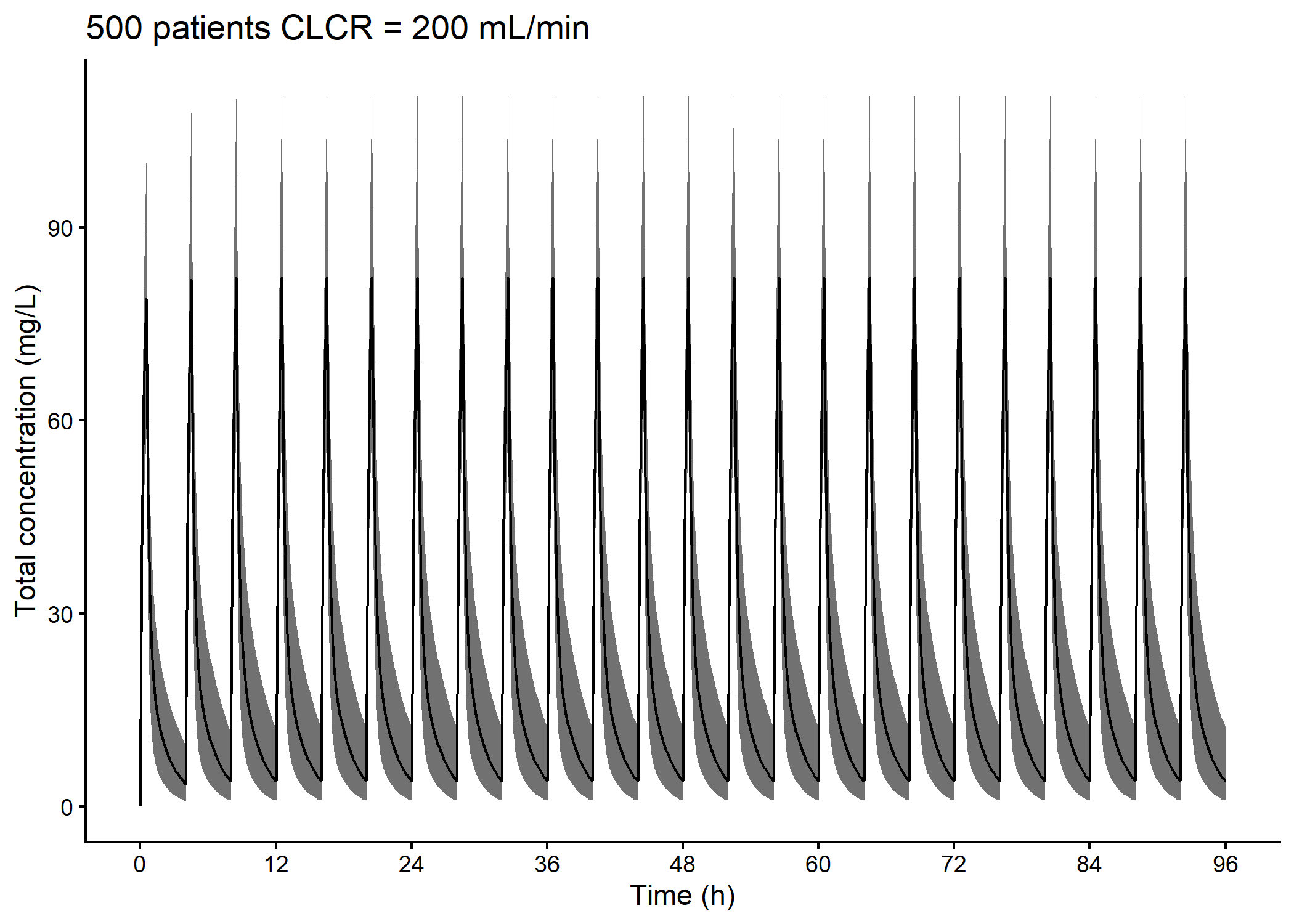
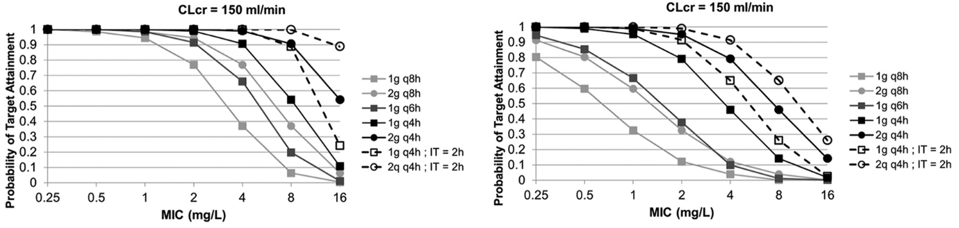
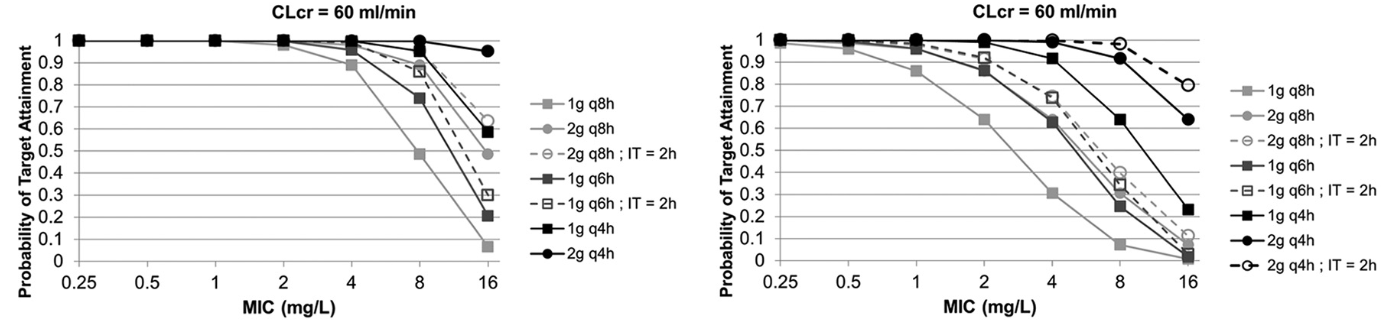
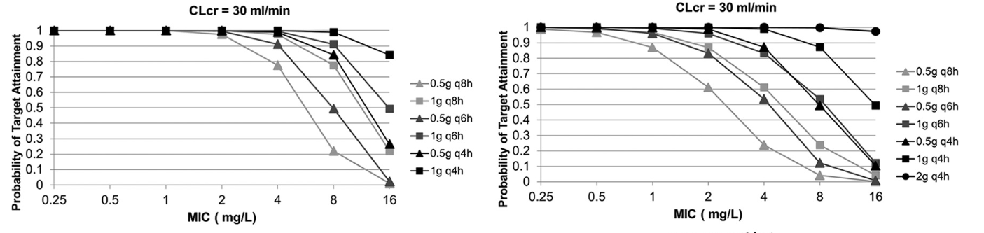
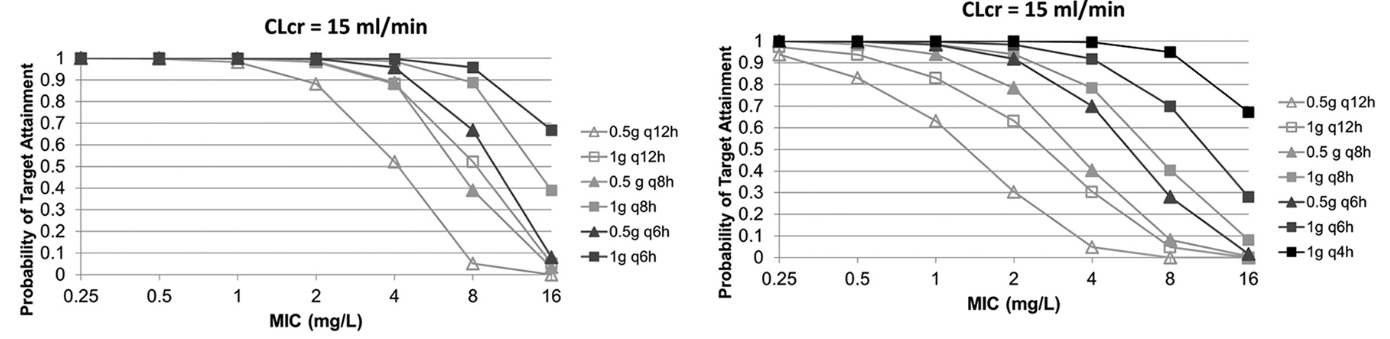
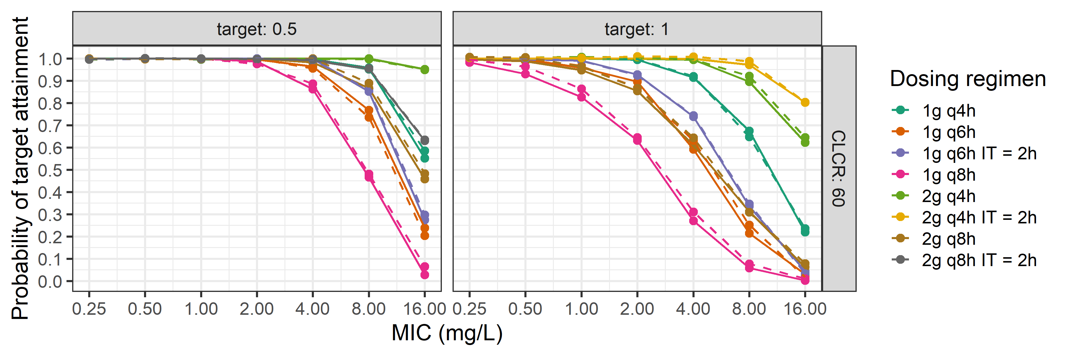
5.2 Reproduction of Figure 4
The figure represents the probability of target attainment for a population of 500 virtual patients of various weight and creatinine clearance, receiving various dosing regimens of amoxicillin. These dosing regimens are represented in the following table :
Patients weights were sampled from a lognormal distribution with mean 89 kg and standard deviation of 0.184 ln(kg).
Show the code
clcr_values <-c(15, 30, 60, 100, 150, 200)creat_values <-convert_clcr_to_creat_cg(clcr_values,wt=70) #convert using mdrd assuming male, 60 yo, and base sizepretty_clcr_values <-paste0(clcr_values, " mL/min")
Simualtions were performed for 6 creatinine clearance values(15 mL/min, 30 mL/min, 60 mL/min, 100 mL/min, 150 mL/min, 200 mL/min)
Show the code
fu <-0.82pkpd_targets <-c(0.5, 1)mics <-2^seq(-2, 4)pretty_pkpd_targets <-paste0(pkpd_targets *100, "%")
Two different fT>MIC (with unbound fraction = 0.82) were studied (50%, 100%). They were computed for a range of MICs (0.25, 0.5, 1, 2, 4, 8, 16 mg/L).
The PTA when the target is 100% of the time above MIC calculated between 10 and 11 simulated days of treatment are inferior to those calculated between 9 and 10 days or 11 and 12 days. In order to reproduce figure 4, PTA were calculated between the 11 an 12th days of therapy.
Show the code
fig4_pta_twelve_days_result_path <- here::here("Model_implementation_validation/data/fournier_2018/sim_results/fig_4_pta_results_twelve_days_of_sim.csv" )# run only if results does not exist yetif (!file.exists(fig4_pta_twelve_days_result_path)) {# Function to #compute PTA for 1 dosing regimen, 1 CLCR, 1 MIC, enables looping through them wrapper_compute_pta <-function(dosing_reg_id, path_dosing_regimens, sim_dur, sim_step, model, patients, path_parameters, cov_default, omega_mat, from, to, targets) { dosing_reg <-select_dosing_regimens(selected_regimen = dosing_reg_id,path_to_the_file = path_dosing_regimens ) sim <-simulate_mrgsolve(dosing_regimen = dosing_reg,sim_dur = sim_dur,model = model,patients = patients,sim_step = sim_step,param_file = path_parameters,cov_default = cov_default,omega_mat = omega_mat ) pta <- purrr::map( targets,~compute_ft_over_mic(sim_tbl = sim,from = from,to = to ) |>compute_pta_t_over_mic(target = .x) ) |> purrr::reduce(dplyr::left_join) |> dplyr::mutate(CLCR = cov_default$CLCR,regimen_id = dosing_reg_id ) pta }#### Dosing regimens to be simulated #### path_dosing_regimens <- here::here("Model_implementation_validation/data/fournier_2018/dosing_regimen_fig_4.csv") dosing_regimens_ids <- readr::read_csv(path_dosing_regimens) |> dplyr::pull(regimen_id) |>unique()#### Patient level covariates #### patients <- readr::read_csv(file = here::here("Model_implementation_validation/data/fournier_2018/simulated_patients.csv"),show_col_types = F )#### PK model, structural and variability parameters #### model <- mrgsolve::mread(model = here::here("Model_implementation_validation/mrgsolve/amox_Fournier.cpp")) path_parameters <- here::here("Model_implementation_validation/data/fournier_2018/model_parameters.csv") eta_CL <-log(0.373^2+1) omega_mat <- mrgsolve::dmat(eta_CL)#### Simulation time parameters #### sim_dur <-288# hours sim_step <-1/6# 1 every 10 min#### PK/PD targets and PTA parameters #### from <-264 to <-288 targets <-c(0.5, 1)#### Setting up the loop for simulations #### regimen_cov_grid <-expand.grid(dosing_reg_id = dosing_regimens_ids,CLCR = clcr_values, # defined in an earlier chunkWT =70, # need a default value, but real value for each patient will be pulled from patients tableMIC = mics, # defined in an earlier chunkSEX =0,AGE =60,BSA =1.73 ) dosing_reg_ids <- regimen_cov_grid$dosing_reg_id cov_list <- dplyr::select(regimen_cov_grid, -dosing_reg_id) |>split(x = _, f =1:nrow(regimen_cov_grid)) model_cov_CLCR <- mrgsolve::mread(model = here::here("Model_implementation_validation/mrgsolve/amox_Fournier_cov_CLCR.cpp"))#### Perform the simulations and compute PTA #### pta_results <- purrr::map2(.x = dosing_reg_ids,.y = cov_list,.f =~wrapper_compute_pta(dosing_reg_id = .x,path_dosing_regimens = path_dosing_regimens,sim_dur = sim_dur,sim_step = sim_step,model = model_cov_CLCR,patients = patients,path_parameters = path_parameters,cov_default = .y,omega_mat = omega_mat,from = from,to = to,targets = targets ) ) |> purrr::list_rbind() |> dplyr::bind_cols(cov_list |> purrr::list_rbind() |> dplyr::select(-MIC,-CLCR)) readr::write_csv(x = pta_results,file = here::here("Model_implementation_validation/data/fournier_2018/sim_results/fig_4_pta_results_twelve_days_of_sim.csv" ) )}
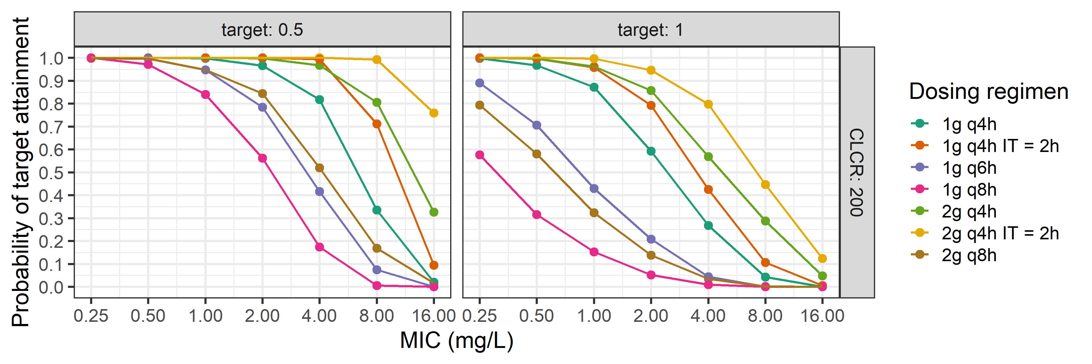
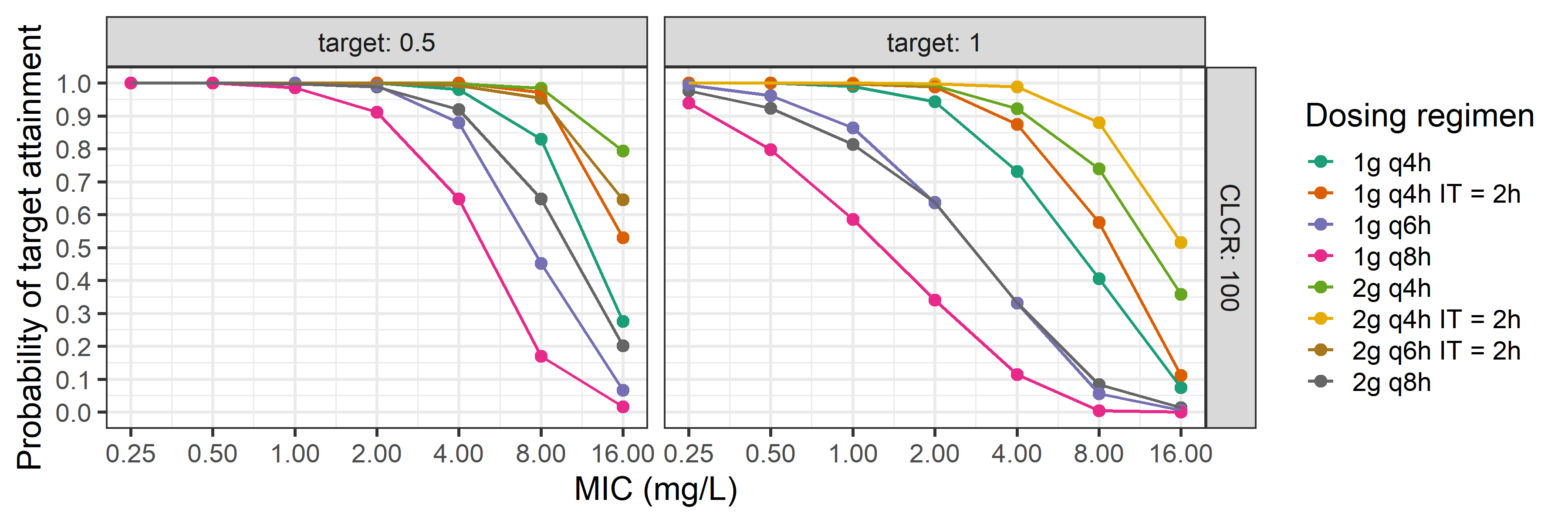
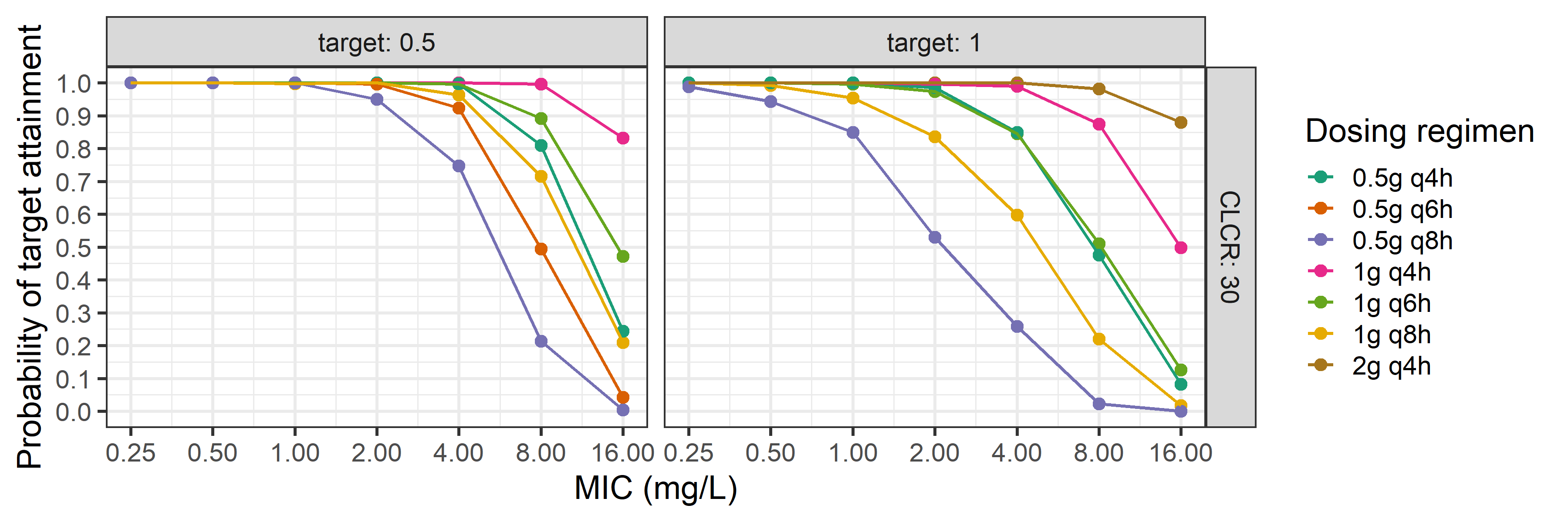
Figure 5.6: Attempt at reproducing the sixth row of figure 4, twelve days of simulation
Regarding over or under estimation of PTA in relation to MIC, compared with PTAs of the original article, no trend can be distinguished. Differences are of the order of 5%. Our simulations line up well with the published figures.
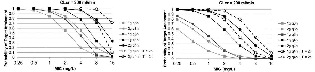
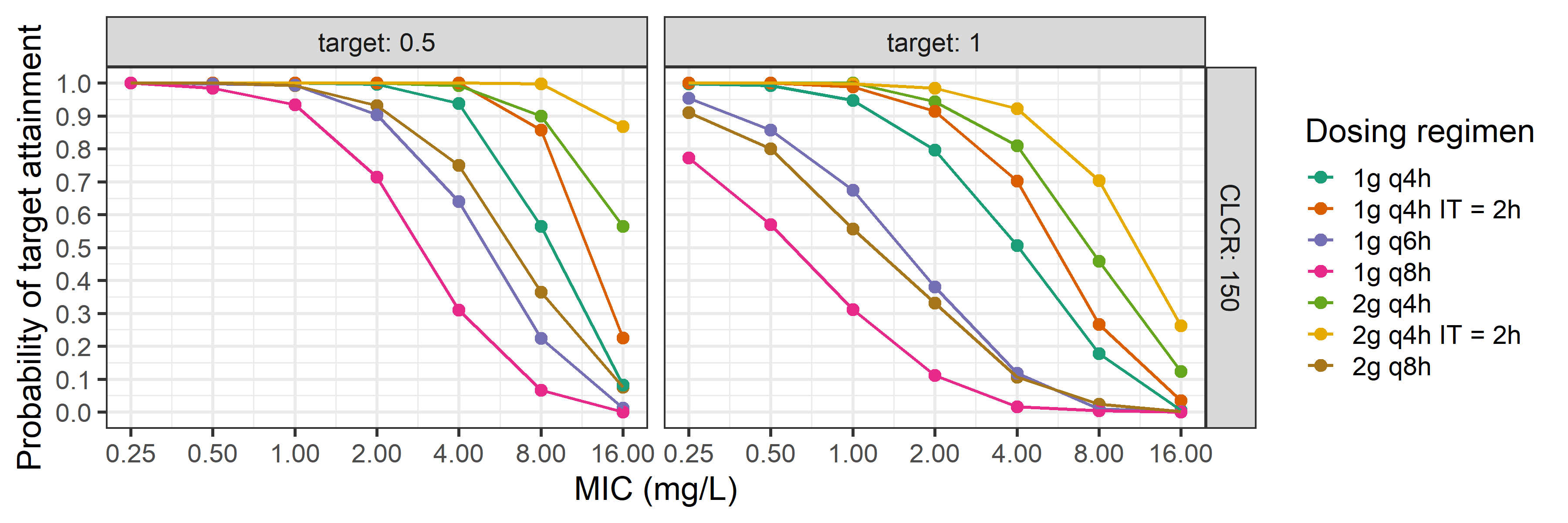
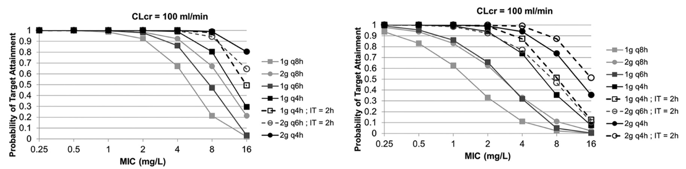
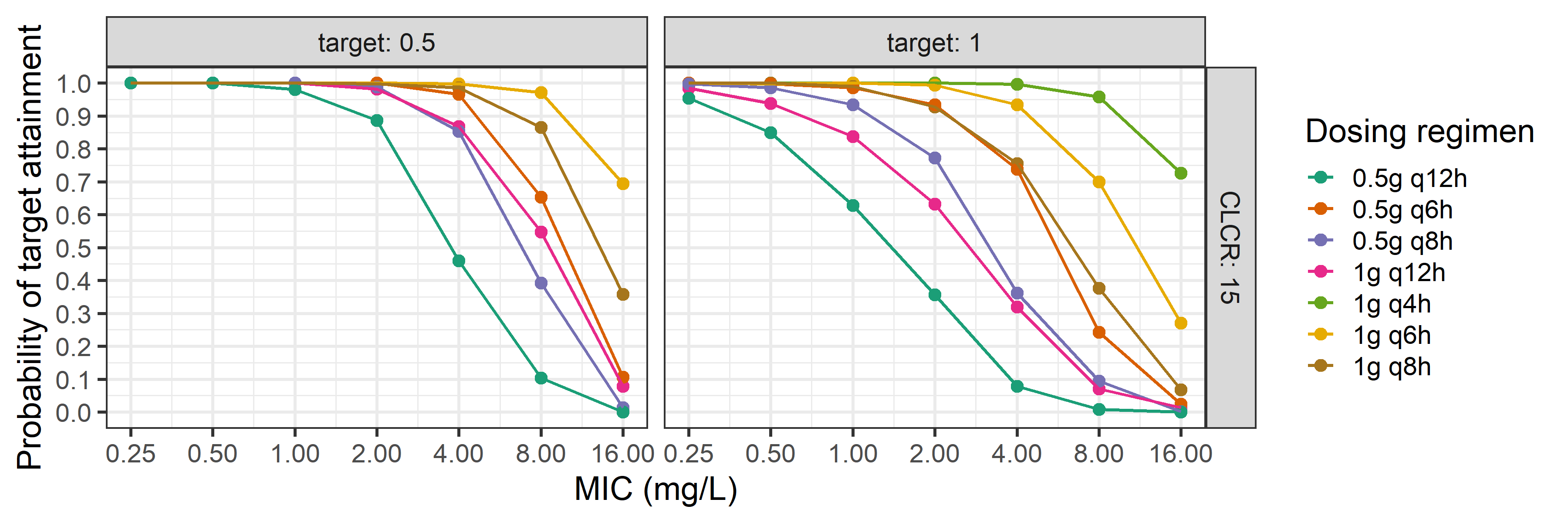
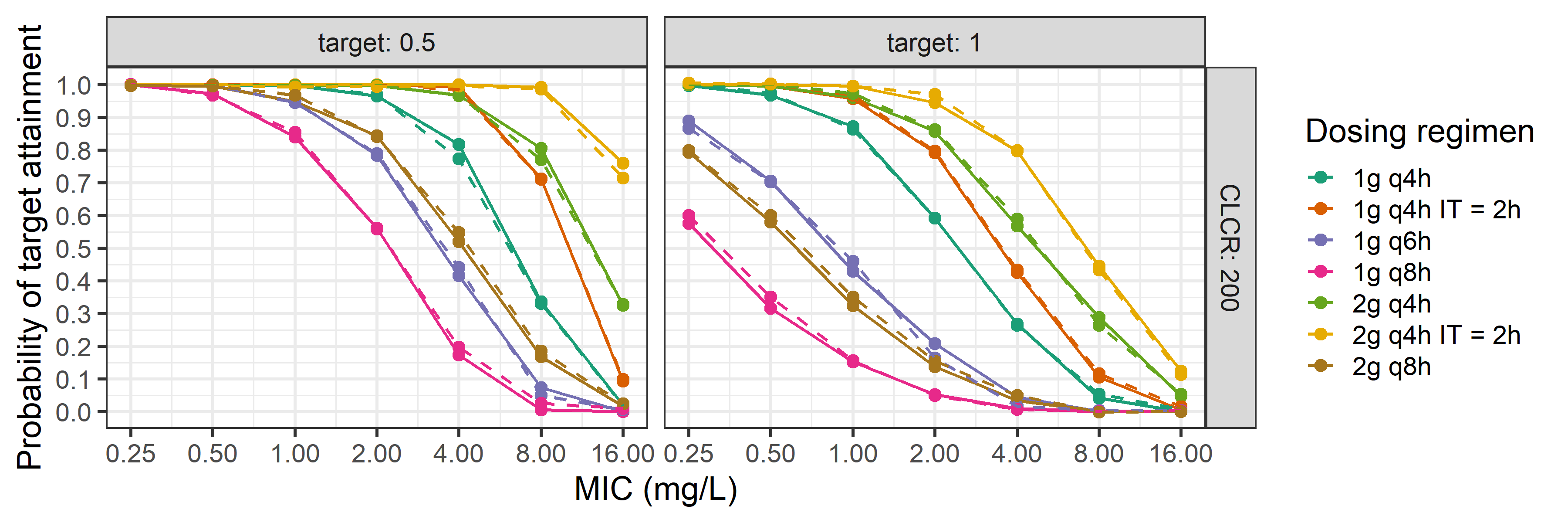
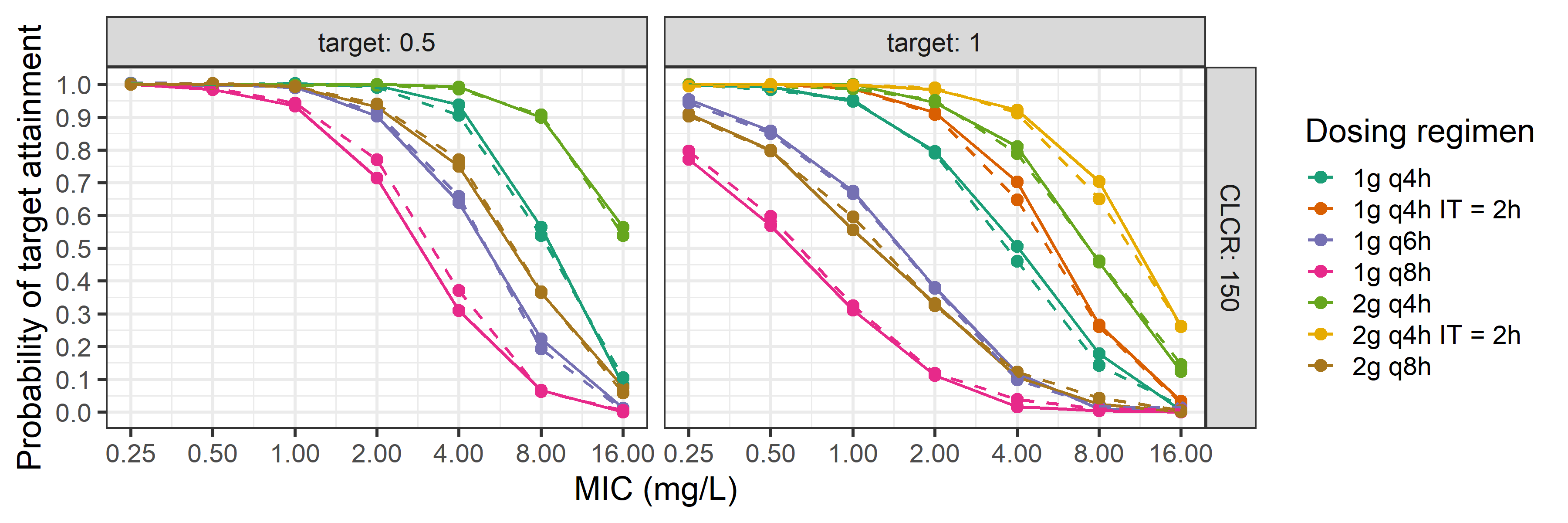
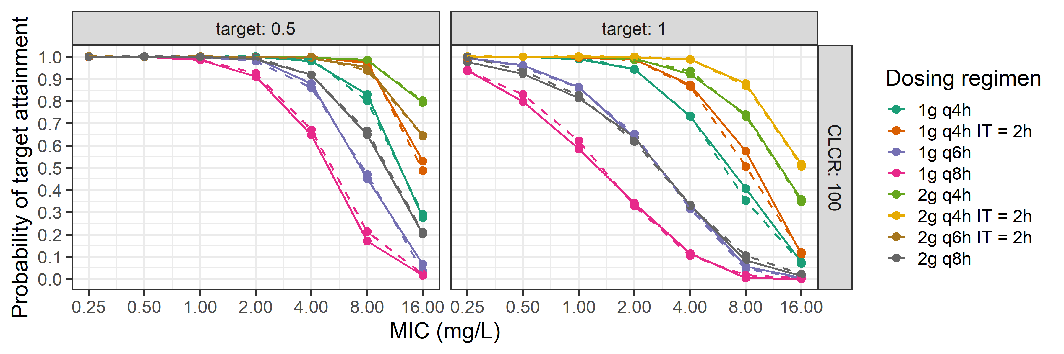
To facilitate comparison between our simulations and the article figure 4, results of our simulations were plotted with article data. Data from the original figure 4 of the article were digitalized. They are the dashed lines in the following figures.
Show the code
# create csv files containing data from article's figure 4 # for each row, one file for PTA 0.5 and one for PTA 1 #### function ##### wanted_pattern has to be written inside quotes # and is the pattern common to the downloaded files joined to form one csv # # csv to write inside data_fig_4# csv_pta_fig_4 = function(wanted_pattern, path_to_new_file) {# files = list.files(path = here::here("../../../Downloads"),# pattern = wanted_pattern)# # pta = purrr::map(.x = files,# .f = ~readr::read_csv(file.path(here::here("../../../Downloads"), .x))) |># dplyr::bind_rows() |># write.csv(file = path_to_new_file)# }# # #### create files ##### # run only if the folder containing digitalized data doesn't exist# if(!file.exists(here::here("Model_implementation_validation/data/fournier_2018/data_fig_4"))) {# # 1st row, left# csv_pta_fig_4(wanted_pattern = "left_1st_row",# path_to_new_file = here::here("Model_implementation_validation/data/fournier_2018/data_fig_4/pta_05_top_row.csv"))# # 1st row, right # csv_pta_fig_4(wanted_pattern = "right_1st_row",# path_to_new_file = here::here("Model_implementation_validation/data/fournier_2018/data_fig_4/pta_1_top_row.csv"))# # 2nd row, left# csv_pta_fig_4(wanted_pattern = "left_2nd_row",# path_to_new_file = here::here("Model_implementation_validation/data/fournier_2018/data_fig_4/pta_05_2nd_row.csv"))# # 2nd row, right # csv_pta_fig_4(wanted_pattern = "right_2nd_row",# path_to_new_file = here::here("Model_implementation_validation/data/fournier_2018/data_fig_4/pta_1_2nd_row.csv"))# # 3rd row, left# csv_pta_fig_4(wanted_pattern = "left_3rd_row",# path_to_new_file = here::here("Model_implementation_validation/data/fournier_2018/data_fig_4/pta_05_3rd_row.csv"))# # 3rd row, right # csv_pta_fig_4(wanted_pattern = "right_3rd_row",# path_to_new_file = here::here("Model_implementation_validation/data/fournier_2018/data_fig_4/pta_1_3rd_row.csv"))# # 4th row, left# csv_pta_fig_4(wanted_pattern = "left_4th_row",# path_to_new_file = here::here("Model_implementation_validation/data/fournier_2018/data_fig_4/pta_05_4th_row.csv"))# # 4th row, right# csv_pta_fig_4(wanted_pattern = "right_4th_row",# path_to_new_file = here::here("Model_implementation_validation/data/fournier_2018/data_fig_4/pta_1_4th_row.csv"))# # 5th row, left# csv_pta_fig_4(wanted_pattern = "left_5th_row",# path_to_new_file = here::here("Model_implementation_validation/data/fournier_2018/data_fig_4/pta_05_5th_row.csv"))# # 5th row, right# csv_pta_fig_4(wanted_pattern = "right_5th_row",# path_to_new_file = here::here("Model_implementation_validation/data/fournier_2018/data_fig_4/pta_1_5th_row.csv"))# # 6th row, left# csv_pta_fig_4(wanted_pattern = "left_6th_row",# path_to_new_file = here::here("Model_implementation_validation/data/fournier_2018/data_fig_4/pta_05_6th_row.csv"))# # 6th row, right# csv_pta_fig_4(wanted_pattern = "right_6th_row",# path_to_new_file = here::here("Model_implementation_validation/data/fournier_2018/data_fig_4/pta_1_6th_row.csv"))# }
Show the code
# regimen_id_pta_05 and regimen_id_pta_1 are character vectors containing dosing regimens for a given creatinin clearance/row and target# path_to_pta_05_article, path_to_pta_1_article are files containing digitalized pTA from figure 4 for this given creatinin clearance/row and targetfig_4_new_plot_row =function(path_to_pta_05_article, path_to_pta_1_article, path_to_results, selected_clcr, regimen_id_pta_05, regimen_id_pta_1) { article_pta_0.5= readr::read_csv(file = path_to_pta_05_article, show_col_types =FALSE) |> dplyr::filter(regimen_id %in% regimen_id_pta_05) |> dplyr::select(y, regimen_id) |> dplyr::rename(PTA_article = y)# add MICs for all dosing regimens to join article and simulated data later # work because digitalized data were sorted by x (MIC) before their export article_pta_0.5_2 = article_pta_0.5|> dplyr::mutate(MIC =rep(c(0.25, 0.5, 1, 2, 4, 8, 16), times = (nrow(article_pta_0.5)/7)))article_pta_1 = readr::read_csv(file = path_to_pta_1_article, show_col_types =FALSE) |> dplyr::filter(regimen_id %in% regimen_id_pta_1) |> dplyr::select(y, regimen_id) |> dplyr::rename(PTA_article = y)article_pta_1_2 = article_pta_1 |> dplyr::mutate(MIC =rep(c(0.25, 0.5, 1, 2, 4, 8, 16), times = (nrow(article_pta_1)/7)))fig_4_row_pta_05_data <- readr::read_csv(file = path_to_results,show_col_types = F ) |> tidyr::pivot_longer(cols = tidyselect::starts_with("PTA"),values_to ="PTA" ) |> dplyr::mutate(target =gsub("PTA_", "", x = name), .keep ="unused") |> dplyr::filter(target ==0.5) |> dplyr::filter(CLCR == selected_clcr & regimen_id %in% regimen_id_pta_05) |>as.data.frame() |>merge(y = article_pta_0.5_2, .by = MIC) fig_4_row_pta_05_datafig_4_row_pta_1_data <- readr::read_csv(file = path_to_results,show_col_types = F ) |> tidyr::pivot_longer(cols = tidyselect::starts_with("PTA"),values_to ="PTA" ) |> dplyr::mutate(target =gsub("PTA_", "", x = name), .keep ="unused") |> dplyr::filter(target ==1) |> dplyr::filter(CLCR == selected_clcr & regimen_id %in% regimen_id_pta_1) |>as.data.frame()|>merge(y = article_pta_1_2, .by = MIC) row_data <- dplyr::full_join(fig_4_row_pta_05_data, fig_4_row_pta_1_data) |> dplyr::mutate(target = forcats::fct_relevel(target, "0.5", "1")) row_data mics =c(0.25, 0.5, 1, 2, 4, 8, 16) row_plot <- ggplot2::ggplot(row_data, ggplot2::aes(x = MIC, y = PTA, color =as.factor(regimen_id))) + ggplot2::geom_point(mapping = ggplot2::aes(x = MIC, y = PTA)) + ggplot2::geom_line(mapping = ggplot2::aes(x = MIC, y = PTA)) + ggplot2::geom_point(mapping = ggplot2::aes(x = MIC, y = PTA_article)) + ggplot2::geom_line(mapping = ggplot2::aes(x = MIC, y = PTA_article), linetype ="dashed") + ggplot2::facet_grid(CLCR ~ target,labeller = ggplot2::labeller(.default = ggplot2::label_both) ) + ggplot2::scale_x_continuous("MIC (mg/L)",transform ="log2",breaks = mics ) + ggplot2::scale_y_continuous("Probability of target attainment",breaks =seq(0, 1, 0.1) ) + ggplot2::scale_color_brewer(name ="Dosing regimen",palette ="Dark2" ) + ggplot2::theme_bw(base_size =18) row_plot}
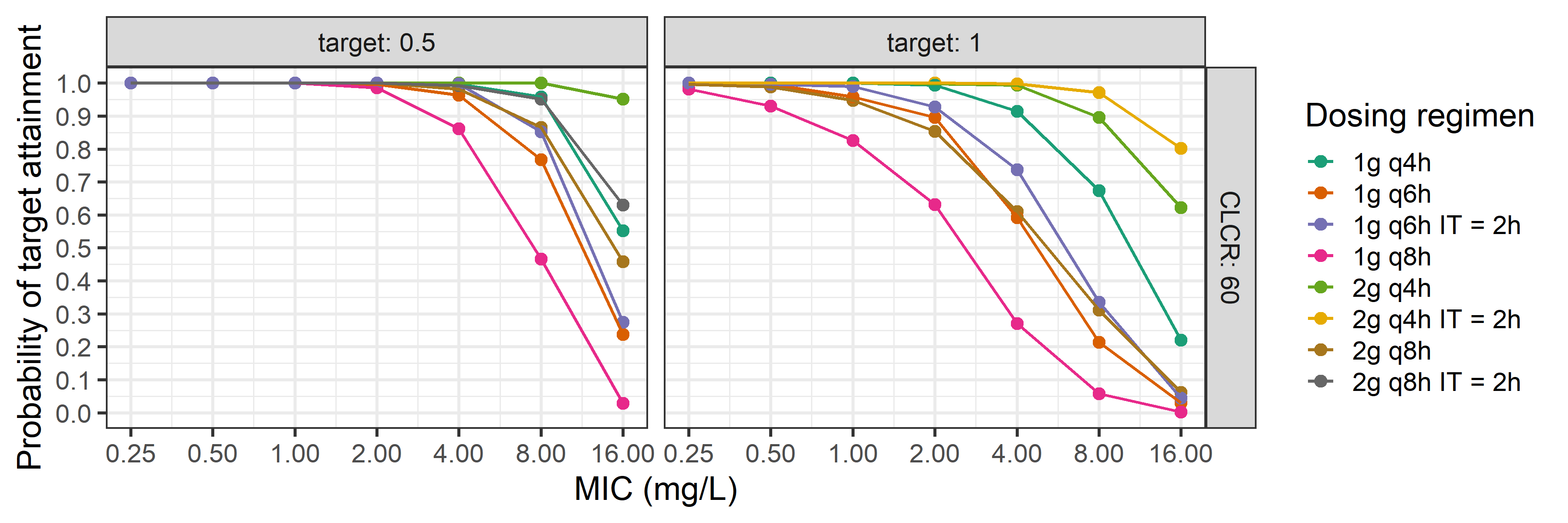
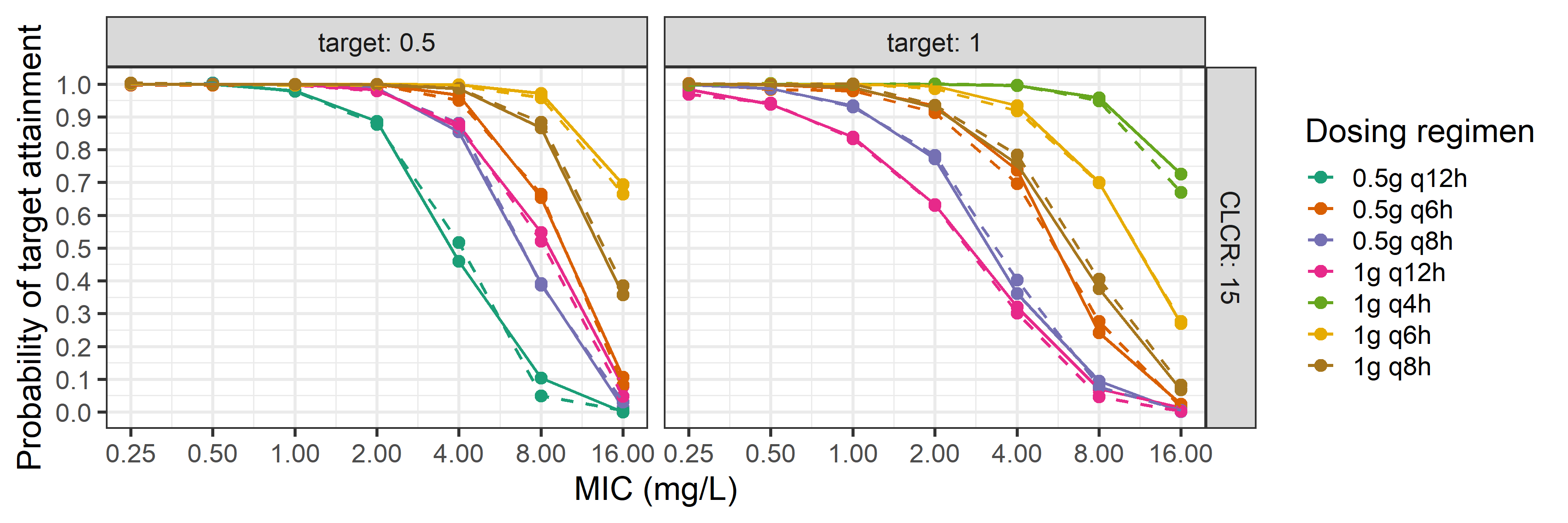
Figure 5.12: Reproduction of the 6th row of figure 4
Regarding over or under estimation of PTA in relation to MIC, compared with PTAs of the original article, no trend can be distinguished. Differences are of the order of 5%. Our simulations line up well with the published figures.
5.3 Reproduction of table 4
Table 4 represents the influence of bodyweight and creatinin clearance on fT>MIC means and PTAs for two targets. Four bodyweight (50, 70, 100, 150 kg) and 3 creatinin clearance were studied. Dosing regimen was 1g infused over 30 minutes every eight hours and MIC was 8 mg/L. For each condition, 500 patients were simulated.
Fournier, Anne, Sylvain Goutelle, Yok-Ai Que, Philippe Eggimann, Olivier Pantet, Farshid Sadeghipour, Pierre Voirol, and Chantal Csajka. 2018. “Population Pharmacokinetic Study of Amoxicillin-Treated Burn Patients Hospitalized at a Swiss Tertiary-Care Center.”Antimicrobial Agents and Chemotherapy 62 (9): e00505–18. https://doi.org/10.1128/AAC.00505-18.